Discrete Optimal Transport

Introduction

Optimal Transport (OT) in its basic form concerns how should one efficiently morph one distribution into another, and the work involved in the morphing is denoted as the distance between the distributions. You might recall the KL divergence as another way to compute distances, however there are some issues with KL, when the intersection of the supports is empty. In this article we I will explain OT for discrete distributions, which is how I first was introduced into the world of OT, specifically through the paper Siddhant and I worked on.

Vanilla Form

Given two discrete distribution $p(x), q(x)$ and a cost matrix $C \in \mathbb{R}^{n \times n}$ our objective can be written as:

\argmin_{\pi \in \mathbb{R}^{n \times n}} <\pi,C> \,\,\,\, s.t. \\ \pi \vec{1} = p\\ \pi^T\vec{1} = q

Note: $\vec{1}\in \mathbb{R}^n$ , is a vector of ones. This is a linear problem, we consequently we can solve this via linear programming. However, if we use methods like Simplex Method, they can sometimes take a lot of iterations to find the optimal. It also turns out that the solutions are sparse. From linear programming, we know that we should be searching for optimal solutions on the vertexs of the polytope. Instead what if we “smoothen” out the problem.

Entropic Regularization

Lets considered a modified objective

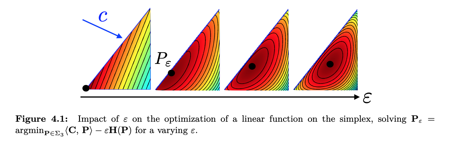
\argmin_{\pi\in \mathbb{R}^{n \times n}} <\pi, C> - \varepsilon H(\pi) \\ H(\pi) \triangleq - \Sigma_{i,j}^n\pi_{i,j}(\log\pi_{i,j}-1)

So we can see that as $\varepsilon$ increases to $\infty$ we are just solving a max entropy problem. Also note that since entropy is convex, our objective still remains convex and we have an optimal solution.

Minimizing the Regularized Problem

If we take the Lagrangian we obtain

L(\pi,\alpha,\beta) = [\Sigma_{i,j}^n[\pi_{i,j}C_{i,j} + \gamma\pi_{i,j}(\log\pi_{i,j}-1)] + \alpha^T(\pi\vec{1}-p) + \beta^T(\pi^T\vec{1}-b)

And from first order optimality we obtain

\nabla_{\pi_{i,j}}L = C_{i,j} + \gamma \log\pi_{i,j} + \alpha_i + \beta_j = 0 \Rightarrow \\ \log \pi_{i,j} = -\frac{C_{i,j}}{\gamma} -\frac{\alpha_i}{\gamma} -\frac{\beta_j}{\gamma} \Rightarrow \\ \pi_{i,j} = e^{-\frac{\alpha_i}{\gamma}}e^{-\frac{C_{i,j}}{\gamma}}e^{-\frac{\beta_j}{\gamma}}

And of course we need to satisfy the marginals summing to $p,q$ . But if we look at the form of the equation for $\pi_{i,j}$ we see that the form of $\pi$ is

\pi = \text{diag}(e^{-\frac{\alpha}{\gamma}})e^{\frac{-C}{\gamma}}\text{diag}(e^{-\frac{\beta}{\gamma}})

Where the matrix/vector exponentials are done element wise. This conveys that we need to find both the diagonal matrices such that $\pi$ satisfies the marginals.

Iterative Bregman Projections

We need to somehow find a way to optimize $\pi$ . First, lets look at our constraints. Specifically, the set of $\pi$ ’s that satisfy the rows summing to $p$ can be written as $A_1 = \{\pi \in \mathbb{R}_+^{n\times n}|\pi\vec{1}=p\}$ , and for the column constraint, $A_2 = \{\pi \in \mathbb{R}_+^{n\times n}|\pi^T\vec{1}=q\}$ . So the set we are interested is $R = A_1 \cap A_2$ . We know there exists a solution to the transport problem (think about moving sand into a hole: Monge) so clearly $R$ is not empty. In addition, $A_1,A_2$ are closed convex sets. Therefore we can look at L.M. Bregman’s paper, The Relaxation Method of Finding The Common Point of Convex Sets and its Application to The Solution of Problems in Convex Programming. A condition for his theorem is we need to find a distance function $D(x,y)$ that satisfies a list of conditions he outlines in the paper. One can show that the KL is a suitable function defined below

\text{KL}(\pi,\xi) \triangleq \Sigma^n_{i,j}\pi_{i,j}(\log\frac{\pi_{i,j}}{\xi_{i,j}}-1)

While this does exactly satisfy the precise requirements, it can be trivially modified (such as non negativity etc). Then we can define a projection as

P_{A_i}^{\text{KL}}(\bar{\pi})=\argmin_{\pi \in A_i}\text{KL}(\pi|\bar{\pi}) = \Sigma^n_{i,j}\pi_{i,j}(\log\frac{\pi_{i,j}}{\bar{\pi}_{i,j}}-1), \pi\in A_i

We can find a closed form via introducing a Lagrange multiplier, and I will assume $i=1$ without loss of generalization

P_{A_i}^{\text{KL}}(\bar{\pi})= \argmin_\pi\Sigma^n_{i,j}\pi_{i,j}(\log\frac{\pi_{i,j}}{\bar{\pi}_{i,j}}-1)-\lambda^T(\pi\vec{1}-p) \Rightarrow \\ \nabla_\pi P_{A_i}^{\text{KL}}(\bar{\pi}) = \log\frac{\pi_{i,j}}{\bar{\pi}_{i,j}}-\lambda_i=0 \Rightarrow \\ \pi_{i,j} = e^{\lambda_i}\bar{\pi}_{i,j}

This implies that the KL projection onto $A_1$ is rescaling the rows of $\bar{\pi}$ such that they sum to $p$ . If $i=2$ , then $\lambda_j$ would appear instead which would imply column scaling. For row scaling, this is equivalent to left multiplying $\bar{\pi}$ by a diagonal matrix, which is equivalent to recalculating $\text{diag}(e^{-\frac{\alpha}{\gamma}})$ . This yields us the Sinkhorn Knopp iterates, where one diagonal matrix is fixed and the other one is updated. Geometrically this is projecting $\pi_t$ onto either $A_1,A_2$ until convergence. Its not hard to show that the updates are

\text{diag}(u)\bar{\pi}\vec{1} = p \Rightarrow \\ u = \frac{p}{\bar{\pi}\vec{1}} \Rightarrow \\ \text{diag}(e^{-\frac{\alpha}{\gamma}}) \leftarrow \text{diag}(e^{-\frac{\alpha}{\gamma}}) \odot \text{diag}(u)

and for the columns

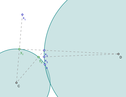
\bar{\pi}\text{diag}(v)\vec{1} = q \Rightarrow \\ v = \frac{q}{\bar{\pi}^T\vec{1}} \Rightarrow \\ \text{diag}(e^{-\frac{\alpha}{\gamma}}) \leftarrow \text{diag}(e^{-\frac{\beta}{\gamma}}) \odot \text{diag}(v)

Geometrically, iterative projections look like the following figure (here the distance metric is Euclidian so the projects are straight, but they don’t have to be as in our case).

Other Related Works

Jason Altschuler has a cool paper [2], which introucdes an alternative variation on the iterates and shows better convergence by showing how the iterates decrease the following potential function.

\Phi(x,y) = \Sigma^n_{i,j}C_{i,j}e^{x_i+y_j}-<r,x>-<c,y>

Here, $x,y$ correspond to the diagonal elements: $e^{x_i}, e^{y_j}.$

References

[1] Computational Optimal Transport

[2] Near-linear time approximation algorithms for optimal transport via Sinkhorn iteration