Euler-Lagrange Equation

A while ago, I saw the Brachistochrone Problem, which is “Find the shape of the curve down which a bead sliding from rest and accelerated by gravity will slip (without friction) from one point to another in the least time.” - Wolfram MathWorld. This problem has a cool answer than involves Calculus of Variations, specifically the Euler-Lagrange Equation which I will explain.

Motivation and Derivation

Moving away from the Brachistochrone Problem, lets look at more general case which encompasses it. We have two times, $t_1, t_2$ , and we have some boundary conditions:

$f(t_1) = x_1, f(t_2) = x_2$ . In addition, we have some objective function which we want to find the local/global min/max. That function is expressed as:

J[f] = \int_{t_1}^{t_2}L(t,f(t),f'(t))dt

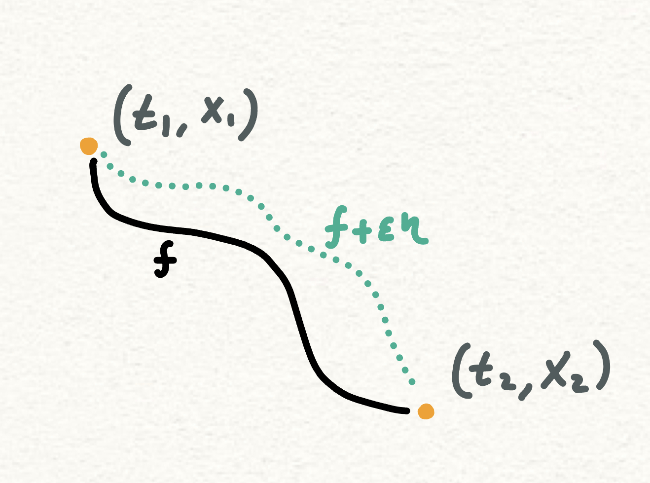
Here $L$ can be any smooth function, in the case of the Brachistochrone Problem it is:

\frac{\sqrt{1+f'(t)^2}}{\sqrt{2gf(t)}}

So lets say $f^*$ is optimal, then in handy wavy terms, we want to some how take a derivative in this functional space and set it to 0. So we need to be able to describe smooth changes to $f^*$ .

f(t)+\epsilon\eta(t)

Here, $\epsilon$ is a scalar value and $\eta(t_1) = \eta(t_2) = 0$ , so varying it along with $\eta$ can explore any function with the same boundary conditions. But the main thing I was thinking about is what lead the creators to add the $\epsilon$ ? Because any function that can be captured by $\epsilon\eta(t)$ can be captured without the use of $\epsilon.$ My current answer to this is: for $f^*$ we want to show that any transition to another function will result in the objective value $J$ becoming non optimal, so to smoothly describe this transition, we can’t just use $\eta$ , since I can’t think of any straightforward way to parametrize all perturbations, since that will require me to somehow control $\eta.$ Instead I can let $\eta$ be anything and control $\epsilon$ . Another perspective is also think of it as an infinite system of equations that we solve at once, where each equation has on particular $\eta$ . This means that when $f = f^*$ then

\forall \eta, \frac{dJ}{d\epsilon}(f+\epsilon\eta) = 0, \text{when } \epsilon = 0.

This is the crux of the Euler Lagrange, the rest of the derivation I feel is more mechanical, and I copied the first and last expression from Wikipedia, you can check the missing details, but they are just regular calculus techniques.

\begin{align} \frac{dJ}{d\epsilon}(f+\epsilon\eta) &= \int_{t_1}^{t_2}\frac{d}{d\epsilon}L(t,f(t)+\epsilon\eta(t),f'(t) + \epsilon\eta'(t))dt\\ &= ...\\ &= \int_{t_1}^{t_2}[\frac{dL}{df}L(t,f(t),f'(t))-\frac{d}{dt}\frac{dL}{df'}L(t,f(t),f'(t))]\eta(t)dt\\ &= 0 \end{align}

Now we initially said that $\eta$ can be anything, so for the integral to equal 0, that means that the expression inside the brackets has to equal 0. You can easily make a counter argument to intuitively see why this has to be the case. Formally it is know as the Fundamental Lemme of Calculus of Variations. This yields us the Euler-Lagrange Equation:

\frac{dL}{df}L(t,f(t),f'(t))-\frac{d}{dt}\frac{dL}{df'}L(t,f(t),f'(t)) = 0

References

https://en.wikipedia.org/wiki/Euler–Lagrange_equation

https://en.wikipedia.org/wiki/Calculus_of_variations

https://en.wikipedia.org/wiki/Fundamental_lemma_of_the_calculus_of_variations

https://mathworld.wolfram.com/BrachistochroneProblem.html