Importance Sampling

Motivation

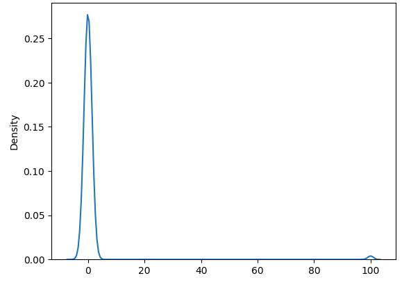
Imagine we have the following GMM distribution, and we want to estimate the expected value via Monte Carlo sampling.

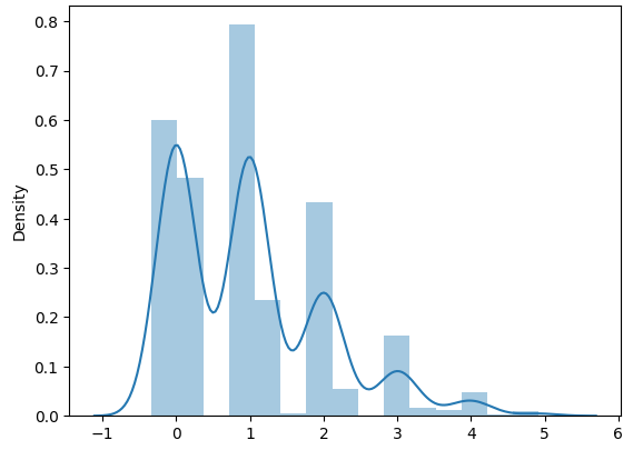
Notice the small hump near 100. This will cause problems when we do Monte Carlo Sampling to estimate the expectation since the majority of the mass is around 0. To illustrate, here is a histogram of 1000 samples of the expectations with sample size 100.

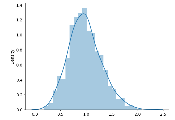
By Central Limit Theorem we know that the distribution should approach a Normal distribution. Which does hold if we increase the sample size to 1000.

So the issue is the high variance induced by the small hump which makes sense because for a low sample size depending on whether we obtain a point from the high value hump or not will change the Monte Carlo Estimation by a decent amount.

Derivation

$\mathbb{E}_p[f(X)] = \int f(x)p(x)dx = \int f(x)\frac{p(x)}{q(x)}q(x)dx = \mathbb{E}_q[\frac{f(x)p(x)}{q(x)}].$ Therefore, if we want to estimate $\mathbb{E}_p[f(x)]$ then we can perform Monte Carlo sampling using $q(x)$ such as $\mathbb{E}_q[\frac{f(x)p(x)}{q(x)}] \approx \frac{1}{n}\Sigma_x\frac{f(x)p(x)}{q(x)}$. We also know that the variance of this is going to be $Var(\frac{f(x)p(x)}{q(x)}) = \mathbb{E_q}[\frac{f^2(x)p^2(x)}{q^2(x)}] - \mathbb{E}_q[\frac{f(x)p(x)}{q(x)}]^2 = \mathbb{E_q}[\frac{f^2(x)p^2(x)}{q^2(x)}] - \mathbb{E}_p[f(x)]^2 = \mathbb{E}_q[(\frac{f(x)p(x)}{q(x)} - \mathbb{E}_p[f(x)])^2]$. Therefore, to set the variance to 0, we can set $q(x) = \frac{f(x)p(x)}{\mathbb{E}_p[f(x)]}$.

However, this only holds if $f(x)\geq0$ for all $x$ in its domain. In addition, while this is the ideal choice of f(x) in reality if you already know the true expected value, then there is no point in this whole thing in the first place ;) Coming back to the non negative problem, it can be shown that $\bar{q}(x) = \frac{|f(x)|p(x)}{c}$ will reduce the variance as well. The proof is taken from the referred source with some of my additional comments.

The main takeaway is; its ideal to make design $q(x)$ such that it puts more weight on the high value humps. Note, the inequality from the Proof comes from Cauchy–Schwarz inequality

References

https://www.math.arizona.edu/~tgk/mc/book_chap6.pdf