Kullback–Leibler divergence (KL divergence)

KL diverges pops up often, for example, your loss function in your neural network might be KL divergence, or if you’re working on variational inference you want to minimize the “difference” between two distributions. Regardless of your application, the KL divergence does the exact thing, somehow measure how different two distributions are. Let’s see how it does it, because it is quite interesting.

Information Theory and Shannon Entropy

I want to first posit this hypothetical scenario. Your friend recently is on an uninhabited island, and they want to transmit the first fish they catch every day. For the sake of this problem, it is given that your friend catches a fish every day.

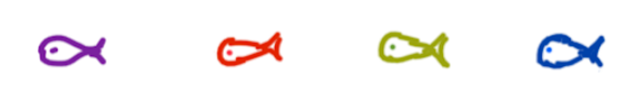
You and your friend know that in the general area there are only four types of fish

Since your friend’s antenna is all set up, you to figure out how to transmit the data efficiently. More specifically, you want to send the least amount of data while not losing any precision. This is where we start diving into Shannon Entropy. Let’s say that after collecting data for 10 days we have a distribution over fish.

Can we use this distribution to create an efficient data transmitting model? Yes, what Claude Shannon figured out is the following set of equations.


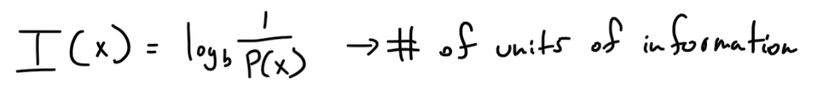
The first equation came arose from a set of criteria Shannon created for information entropy, you can read about them here. Let’s understand what this equation means. It’s calculating the information of an event. The base of the logarithm repersents what unit of information your working with, since we are going to use binary we will use 2. So the information of an event is the minimum number of bits needed to encode that event. So if there was only one type of fish, then every day your friend will catch the exact same fish, so you might as well not even read the data he sent you since it conveys no useful information. This is verified by the equation, since log(1)=0, which means you need no bits.

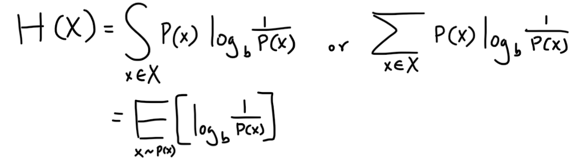
The second equation is the entropy for the distribution, which is the expected value of the information (number of bits). A uniform distribution would have the highest entropy since you have no clue which event it’s going to spit out.

Hypothetically, lets say there are two distributions, which will help illustrate certain ideas.

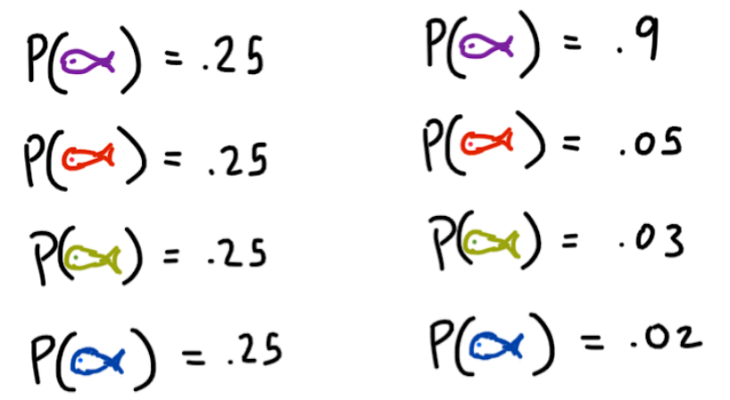
So let’s take the one on the left distribution, it is saying that each fish is equally likely. Thus I(purple) = I(red) = I(green) = I(blue) = 2, which means that at least 2 bits of information are needed to encode each type of fish. We will get into the actual encoding a bit later. For the distribution on the right, we can see that the purple fish is most likely, and consequently, the information that it conveys is lower. I(purple) = 0.15. And for the remaining fish, I(red) = 4.32,I(green) = 5.05, I(blue) = 5.64.

Huffman Coding

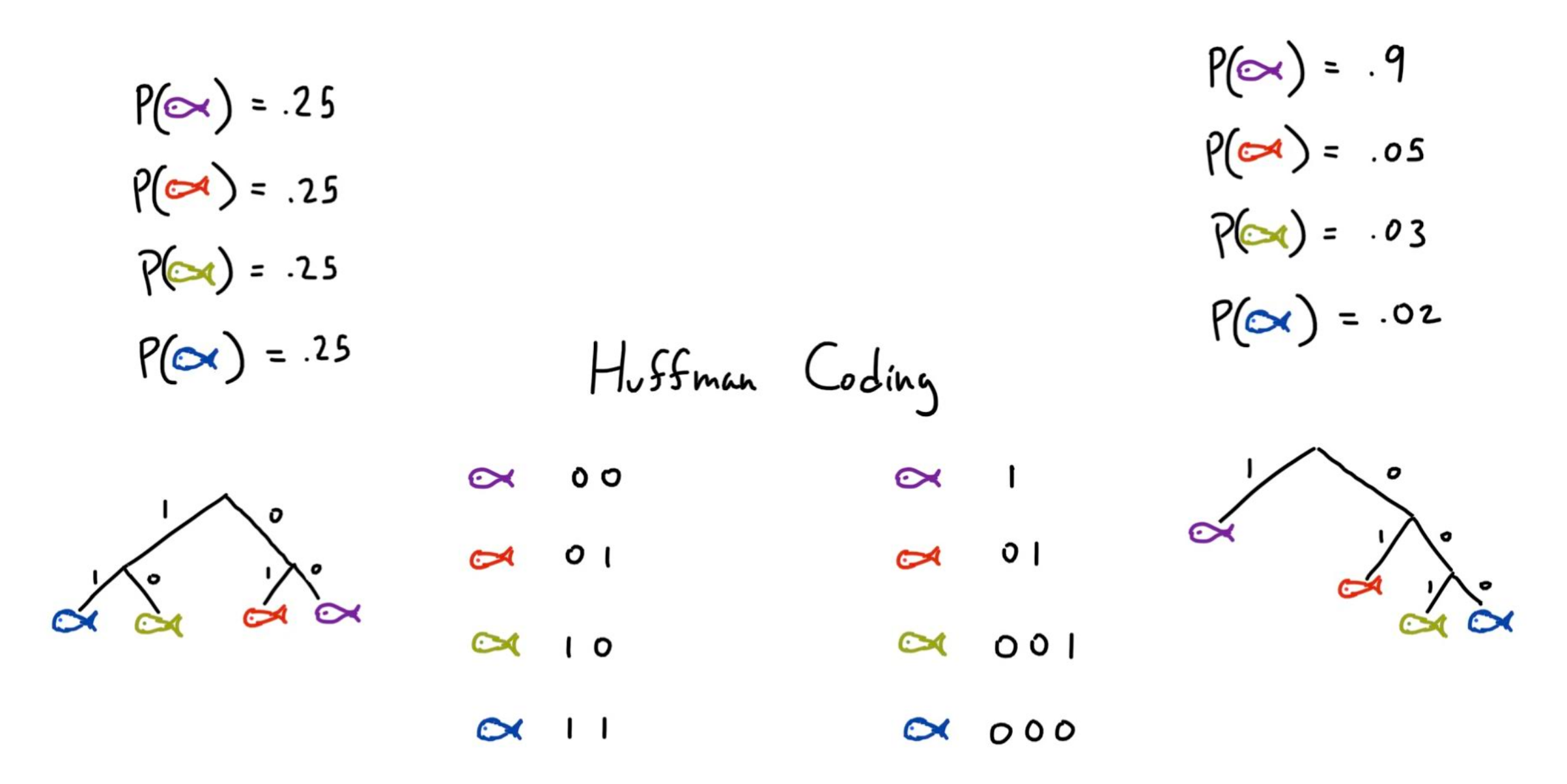
Huffman Coding creates a graph based on a distribution, where the expected value of the path is minimized. In this case, since we are working with bits, we will have a binary tree, and using an online Huffman Coding calculator, we can generate the Huffman Coding for each distribution. Notice that for the uniform distribution, the one on the left, the tree is full at each level, this should make sense since we needed 2 bits for each event. However, for the distribution on the right, the purple fish is very likley, so you would want to minimize the number of edges needed, which is the number of bits. Thus we at the top of the tree, with one branch.

KL Divergence

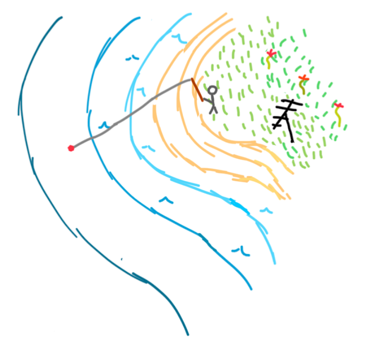
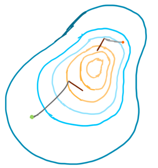
I think the best way to convey KL Divergence, is to provide a modification to our original scenario. Shown in the image below, our friend now has two fishing locations, one on each end of the island, and each is cast to a different depth in the ocean.

Now based on what we have learned so far, we would need two distributions, on for the orange location and one for the green location. Let’s say our following two distributions are the ones below.

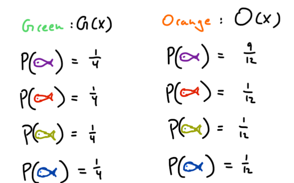
Everything seems, fine, we have two separate distributions, one for each location, and say our friend sends the result of each fishing line at specific agreed upon time, so there is no ambiguity. To convey KL divergence, let’s say our friend made a mistake. They used the Orange location’s distribution to transmit the fish at the Green location. Yikes! This is going to cost us in terms of efficiency. But how much is this going to cost us? This is what KL Divergence answers. Take a look at the following expression.

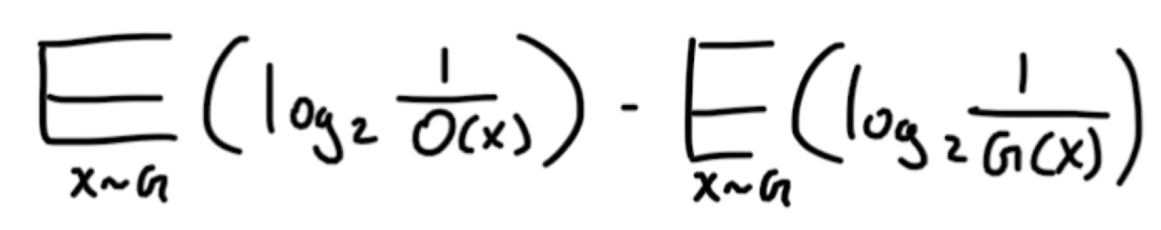
The first term represents the expected length of information (bits in our case) of using the Orange location’s distribution at the Green location. The second term is the normal expected value of the Green location’s information. So taking their difference is equal to the number of extra bits being used, which is also known as the information gain. Let’s simplify our expression via the following steps.

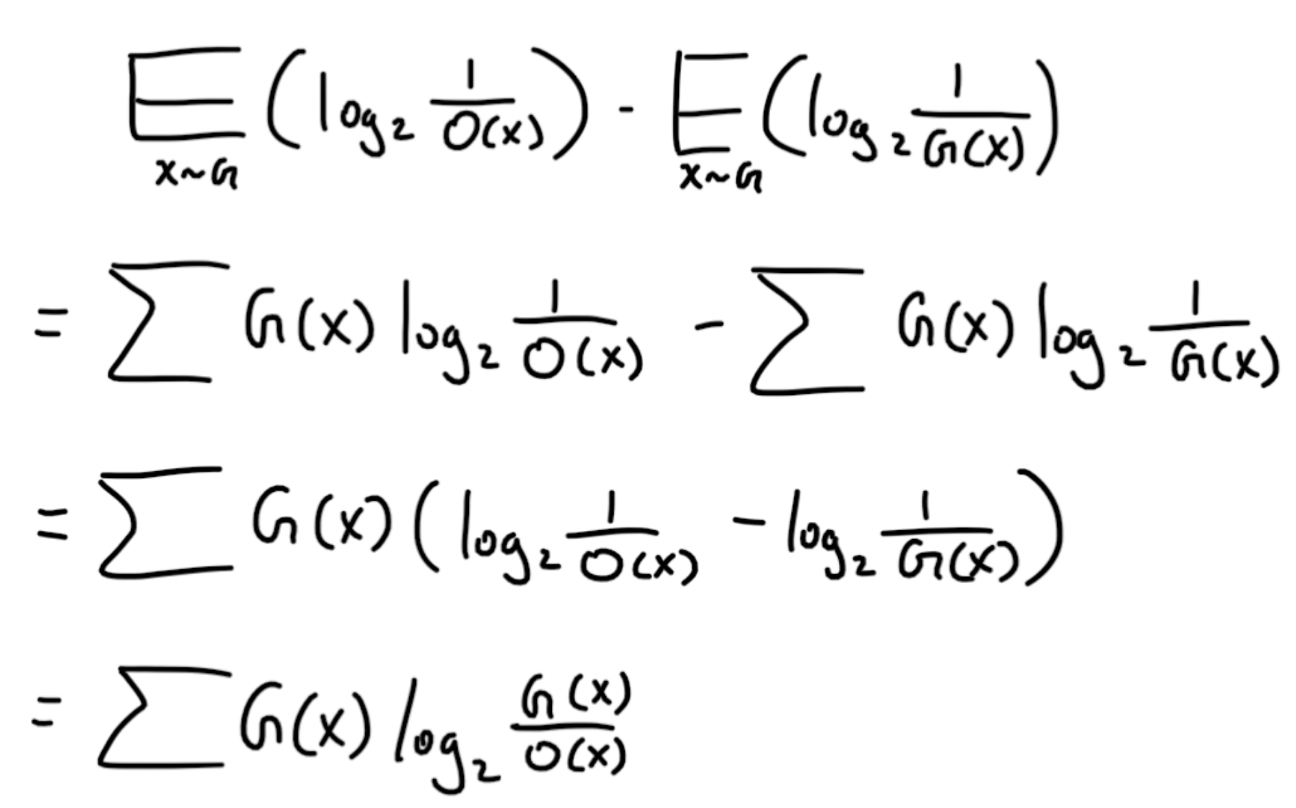
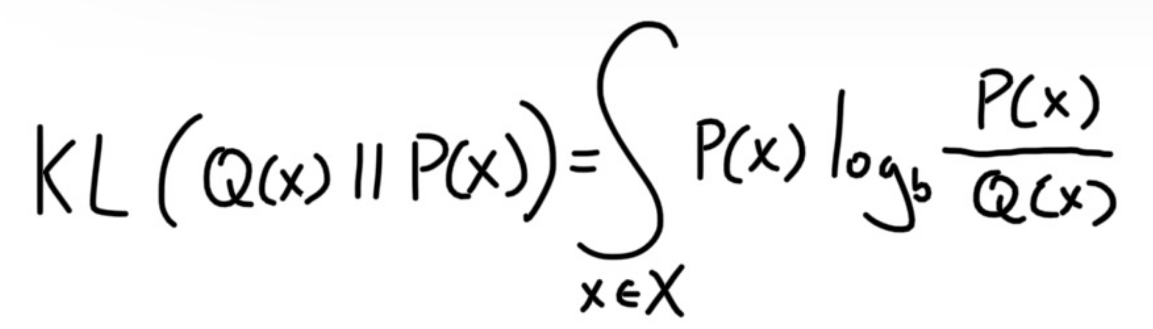
We have arrived at the KL divergene formula for the discrete case, for a continous distribution, it is the following

That’s all, thanks for reading!

References

https://brilliant.org/wiki/entropy-information-theory/
https://en.wikipedia.org/wiki/Huffman_coding
https://en.wikipedia.org/wiki/Kullback%E2%80%93Leibler_divergence
https://planetcalc.com/2481/