Lagrange Multiplier
We see maximization or minimization problems often. In most of those problems, we need to find any (x,y)
such that f(x,y) is maximized or minimized. However, what if (x,y) can’t be any value from dom f(x,y)? This is where Lagrange Multipliers come in. Note, in this article, I only refer to f as being a function of two variable, but this idea is applicable for all functions
One Perspective
Let’s start with a problem to illustrate the inner workings of the Lagrange Multiplier. We have the functions
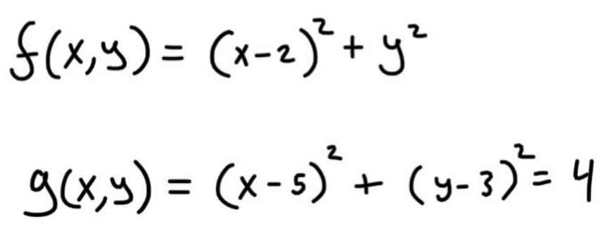
f(x,y) is what we want to find the critical points of, and g(x,y) is our constraint. I made the functions simple, so the contour plots are simple. Contour plots, how are those related? Take a look a the following image.
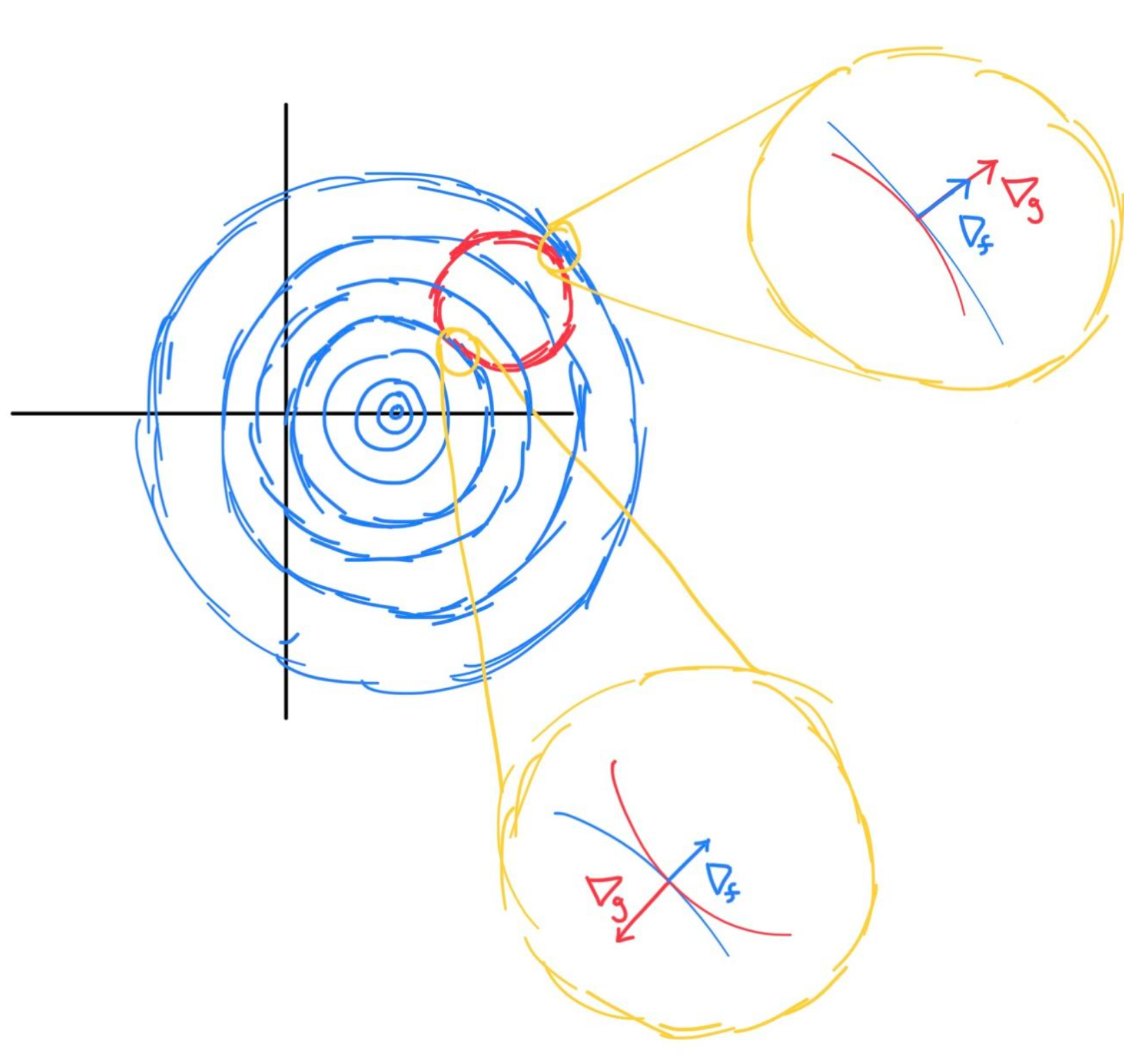
In your head, visualize the animation of the contour as you slice f(x,y) by the plane . That plane will interest
f in one spot, thus the contour is just a dot. However make the plane shift up a little, so it becomes , you will obtain a tiny circle. So we can say to find the minimal value of
f constrained on g, we need to find the smallest value c such that just touches our constraint which is the red circle. Therefore, both curves would be tangent to each other, which is why their gradients will have the same direction, but different magnitude. To understand why the gradient is perpendicular to the contour, observe the following equations. The first equation is the directional derivative of the contour.
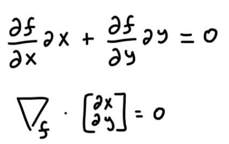
Since the dot product between the gradient and the contour vector is 0, that means both vectors are orthogonal. Coming back to our problem, since both curves share the same contour direction, their gradients will also point in the same direction. This means we can set the gradients equal to each other if we scale one of them. The scaling factor is the Lagrange Multiplier. To generalize, for any critical point on f constrained on g, the contour of f at that point will be tangent to the contour of g. Think about this, since it’s a very interesting idea. We can now understand the first equation from the following image.
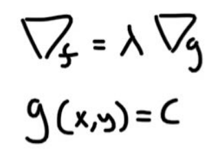
The second eqation, is just our consraint. So now we have enough equations and variables to solve for (x,y).
Another Perspective
There is another way to look at this constrained optimization, and I see this approach more oftenly used. The following equation is called the Lagrangian.
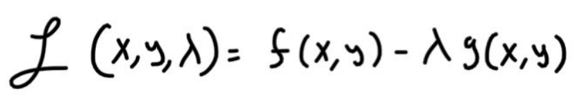
In this form, its required that our constraint, . This means that for all
(x,y) not satasifying the constarint, f(x,y) will be lower by . To get a visual understanding, keep imaging
, increasing, and thus the critical points start forming mounds and eventually peaks. Therefore, to use the lagrangian we just need to find
such that
. If you carry out the partial derivatives, you will find the yourself arriving at the same set of equations in the first perspective.
The Catch
This method can fail for one edge case, and that’s when , read this great article to get a full explanation.