Langevin Sampling

Intro

Langevin sampling is another sampling technique that just requires that you can compute $\nabla \log p(x)$ . Specifically, it constructs an Stochastic Differential Equation (SDE) such that the stationary distribution is $p(x)$ . Lets look into the theory of how a random walk can sampling a distribution.

Itô Calculus and Fokker-Plank Equation

Let $B_t$ be Brownian motion. So $B_0 = 0$ , and $B_{t_2} - B_{t_1} \sim N(0,t_2-t_1), t_2 > t_1$ . Consider $dB_t$ . This isn’t the usual calculus definition of a change of a function, in fact it can be shown that $\frac{d}{dt}B_t$ doesn’t exist, and it makes sense intuitively, its a distribution, so it won’t converge to some exact value. But Itô made an interesting observation.

lim_{n\rightarrow\infty}\Sigma_i^n(B_{t_{i+1}} - B_{t_{i}})^2 = T

Where, $t_i$ are equidistant points from $0$ to $T.$ What this tells us is that $(dB_t)^2 = dt$ . This leads us to Itô’s lemme which states that for $f(x,t):\R^2\rightarrow \R$

df = \frac{\partial f}{\partial t}dt + \frac{\partial f}{\partial x}dx + \frac{1}{2}\frac{\partial^2 f}{\partial x^2}dx^2

Where $x$ follows a stochastic process, which is why $dx^2$ doesn’t vanish. You can derive this by doing a Taylor expansion and then removing the terms that vanish. Lets specify the stochastic process for $x$ :

dx = \mu(x,t)dt+\sigma(x,t)dB_t

substituting $dx$ into the expression for $df$ yields:

(\frac{\partial f}{\partial t} + \frac{\partial f}{ \partial x}\mu(x,t))\partial t + \frac{\partial f}{\partial x}\sigma(x,t)dB_t + \frac{\partial^2 f}{\partial x^2}\mu(x,t)\sigma(x,t)dtdB_t + \frac{1}{2}\frac{\partial^2f}{\partial x^2}\sigma(x,t)^2dB_t^2

and after taking the expectation over $x$ which is based on the true distribution of $x$ at time $t$ , $p(x,t).$ The terms with $dB_t$ disappear and after doing some algebra we get the Fokker-Plank Equation. I like the proof in this article if you want to look at the details.

Fokker-Plank Equation

\frac{\partial p}{\partial t} = -\frac{\partial}{\partial x}(\mu(x,t)p(x,t)) + \frac{1}{2}\frac{\partial^2}{\partial x^2}(\sigma(x,t)^2p(x,t))

So ideally we want $lim_{t\rightarrow \infty}p(x,t)$ to converge to $p(x)$ which is the original distribution we wanted to sample from. So we can agree that as time limits, then the partial derivative with respect to time should equal $0$ , which would imply that the distribution converges. It can be shown that the following stochastic process does have our desired stationary distribution.

dx = \nabla_x\log p(x)dt + \sqrt{2}dB_t

I recommend this well written article to see why that is the case.

Implementation

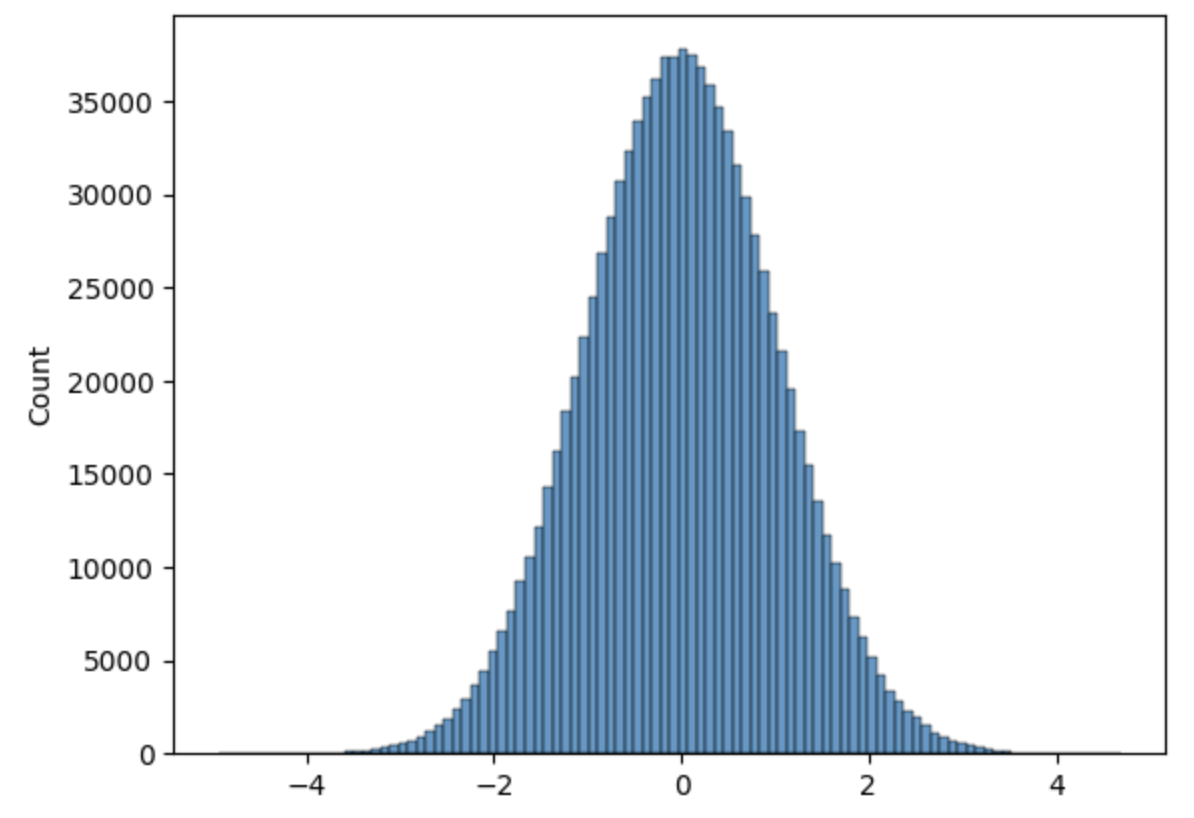
Here is a short code to sample a standard normal distribution.

import matplotlib.pyplot as plt
import numpy as np
import math

def pdf(x, mu, sigma):
    # gaussian pdf 
    return (1/(sigma*math.sqrt(2*math.pi))) * math.exp((-1/2)*((x-mu)/sigma)**2)

def pdf_deriv(x, mu, sigma):
    return (-1/((sigma**3)*math.sqrt(2*math.pi))) * math.exp((-1/2)*((x-mu)/sigma)**2) * (x-mu)

# take on step of the Monte Carlo Process
def step(x, a, mu, sigma):
    # taking the gradient of ln(pdf) = 1/pdf * pdf_deriv
    return x + a * (1/pdf(x, mu, sigma))*pdf_deriv(x, mu, sigma) + math.sqrt(2*a)*np.random.normal(0,1,1)[0]

x_vals = []
x = 1
alpha = 0.1
num_iter = 1000000
for i in range(num_iter):
    x_vals.append(x)
    x = step(x, alpha, 0, 1)

plt.hist(x_vals, bins=100)
plt.show()

As expected we obtain the standard normal.

References and Resources

https://www.thphys.uni-heidelberg.de/~wolschin/statsem21_6s.pdf

https://abdulfatir.com/blog/2020/Langevin-Monte-Carlo/

https://www.youtube.com/watch?v=Z5yRMMVUC5w&list=PLUl4u3cNGP63ctJIEC1UnZ0btsphnnoHR&index=17