Model Merging
This is going to be a more exploratory post on a splatter of interesting ideas from multiple papers discussing model merging. Model merging is a very interesting topic because the idea of taking model trained on different distributions and somehow using them to create a new model that can operate over both distributions is fascinating.
Why Merging?
Given the recent popularity of LLMs and their impressive capabilities, users are effectively finetuning these models on smaller datasets to elicit custom behaviors. So now we have many finetuned checkpoints floating around, and so, one can ask: could we somehow combine all these checkpoints into a mega model that has all the capabilities from the individual checkpoints? Sounds amazing if true, and it is partly true!
Main Resources
This post is going to mainly be talking about ideas explained in the following posts / papers. It may be good to read them first to give a better context.
Papers:
Core Concepts:
 https://agustinus.kristia.de/techblog/2018/03/11/fisher-information/
 https://agustinus.kristia.de/techblog/2020/11/02/hessian-curvatures/
 https://en.wikipedia.org/wiki/Laplace's_approximation
Preliminary
Typically model merging is posed using the following formulation.
Consider we have a base model and datasets . Then is separately trained on yielding, . Since the architecture of doesn’t change during training, we can just consider the trained parameters . Now, we want to obtain a single which is the optimal parameter such that is able to perform well on .
A simple approach, averaging.
Indeed, averaging is a commonly used method, where . The federated averaging community uses this quite often, known as FedAvg.
Can curvature help us?
If all we have access to is, , then there isn’t too much we can do. However, what if we start to extract more information, like understanding the model’s sensitivity to different parameter dimensions? To more concretely view this, consider to be a likelihood model, that is, . Now if we look at the posterior, , we can frame the problem of finding the parameters that is best at solving as the following
This yields, . However, the assumption we made was the posterior can be approximated by an Gaussian distribution with unit covariance. However, we know that it is likely that the shape isn’t going to be isotropic. So here we can utilize the Laplace approximation for the posterior, which I linked above. In essence, it is also trying to approximate the posterior distribution with a Gaussian distribution, but not with an isotropic one. Instead we will look at the second order characteristics of the distribution to shape the covariance matrix. Specifically, the Laplace approximation models the posterior as:
I am going to take a small detour now to talk about something we will use a bit later, the Fisher information matrix. First we define the score function as, . It can be shown that
. Using this, we can also look at the covariance which yields the Fisher information matrix
It turns out that under the modes of the distribution, we can substitute, where is the Hessian for the Laplace approximation see [Perone et al]. Then we can revisit the original objective, and update it to the following
In practice usually only the diagonal of the Fisher is used for computational efficiency, and so each merged parameter dimension is scaled by the normalized Fisher diagonal values, the authors a closed form solution:
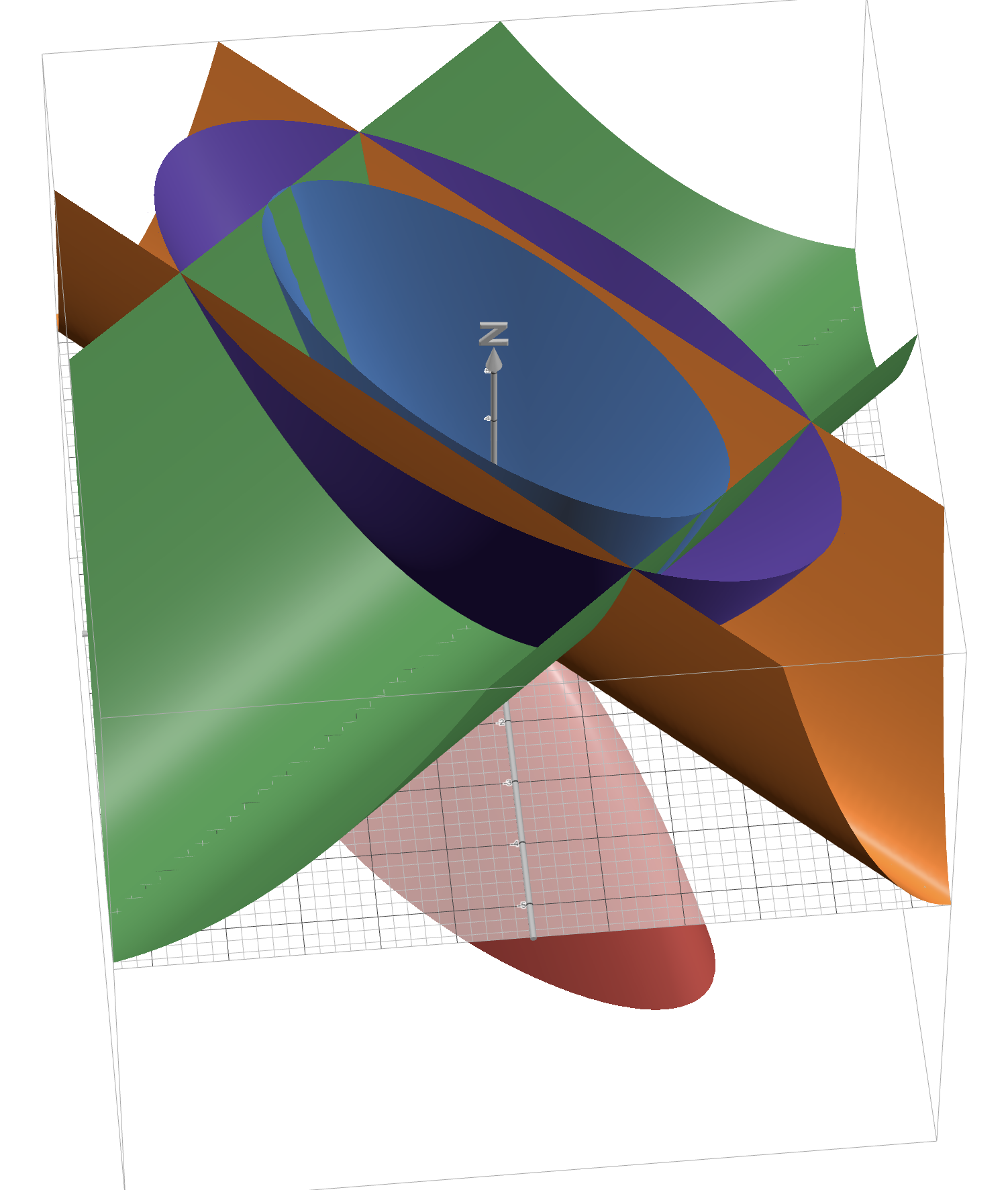
As a mental exercise think about the intuition behind this, for parameters that have a high Fisher information, we would want them to be less changed when averaging, whereas the low Fisher information values can be changed more without as much degradation in the performance. And try to draw the connection in terms of curvature in a quadratic function like , we wouldn’t want the move too far away from the principle axis of curvature (the eigen vector of that corresponds to the larger eigen value of . In addition, geometrically (disclaimer this is handy wavy and just how I got a visual understanding, this is not rigorous at all) if we look at ellipsoid quadratic equation, and their negative version , we can see you get a quadratic ellipsoid with that is flipped across the domain plane. Then if we look at samples, we can see that it too will form an ellipsoid with the same principle axis. Then when we take each and make a rank 1 matrix if we then look at a quadractic form this takes, via plotting , then we can see it forms a trough shape. Then we just plot both trough’s that correspond to the principle axis, and when we combine both plots we roughly recover the negative hessian plot. These values are eye balled, so it won’t be exact lol.
Another angle is Task Arithmetic (TA), and the paper from [Daheim et al] describes cool analysis on it. Consider the details of the loss function typically used. In that we optimize for the task loss for task , and we have a weight regularization .
A cool equation they show is what are the errors when performing TA, what if we want to merge the parameters with weightings on the task given by , we can see what does the difference between the optimal parameter which is given as
Where, are the weights of some pretrained model that we don’t want significantly diverge from, and Mahalanbois distance, which is a quadratic distance, is used as the regularizer. . And the TA merged parameters which are
So how does, compare to ? Turns out we can derive the difference to be!
Then we can Taylor expand, , where is the Hessian. Then
So it shows that under the Taylor approximation, we should be utilizing the Hessians to shape how we merge the “task vectors”
This starts to elude to the final paper[Tam et al] which I will briefly discuss here which says that a general perspective to see model merging is
Where is an “(approximate) covariance matrix of some random variable”. And depending on how you set you can model common techinques like Simple Averaging, Fisher Merging . This goes to show that we really are warping the parameters under a linear transfirmation and reweighing them. I won’t go further into that paper’s details, but do check it out. I mainly wanted to end on this because it is interesting to think about what if we move beyond the general framework they presented. Thanks for listening, and feel free to shoot me an email if there is a mistake / if you want to see other topics covered.