Metropolis Hastings (MH)
Sampling from a high dimensional distribution is hard. To illustrate this, say we have the following distribution that we want to sample from: P(a,b,c,d). We can rewrite it as P(A=a)P(B=b|A=a)P(C=c|B=b,A=a)P(D=d|C=c,B=b,A=a). Sampling the first term A is hard, it requires that we marginalize over 3 variables! Therefore, faster approaches have been developed to solve this problem, MCMC being a prominent high-level technique. Metropolis-Hastings is a type of MCMC approach.
Detailed Balance Equation
The detail balance equation is a very important concept for MH. Say we have a probability distribution P. The detailed balance states that if we can construct a Markov Chain, whose transition probability is T(xi|xj), then, for all xi and xj, if the P(xj)T(xi|xj) = P(xi)T(xj|xi), then the Markov Chain’s stationary distribution is equal to P.
The Metropolis Hastings Equation
Proposal Distribution
First, define a proposal distribution Q(xi|xj). This distribution proposes candidate samples. In this post, I will only talk about symmetric distributions for Q, more specifically I will let Q be the normal distribution. Lets define Q(xi|xj) = N(xi|μ=xj,∑=1), and it should be clear why Q(xi|xj) = Q(xj|xi).
Critic
The final aspect of MH, is the critic. It will tell you the probabilty at which we should accept a proposed sample, produced by the proposal distribution. Lets denote this as A(xi|xj). Now we have defined all the aspects of MH, we can write T(xi|xj) = Q(xi|xj)A(xi|xj) for all xi != xj, if xi = xj then T(xi|xj) = Q(xi|xj)A(xi|xj) for all possible xj sum Q(xi|xj)(1-A(xi|xj)). We will mainly refer to the case when xi = xj since its easier to write, but the following equations will still hold if xi != xj. With all this said, we still don’t know how to calculate A, our critic probability. Recall the detailed balance equation, we can expand to be: P(xj)Q(xi|xj)A(xi|xj) = P(xi)Q(xj|xi)A(xj|xi). We can shuffle some terms around to produce this equation A(xi|xj)/A(xj|xi) = P(xi)Q(xj|xi) / P(xj)Q(xi|xj). The following information im going to explain is probably the most confusing. For every itteration where we sample Q given our current location, xj, and obtain the proposed sample, xi. We want to figure out A(xi|xj), so what we can do is set A(xj|xi) = 1 when P(xi)Q(xj|xi) / P(xj)Q(xi|xj) < 1. However, if P(xi)Q(xj|xi) / P(xj)Q(xi|xj) > 1 then A(xi|xj) = 1. I think its important that you think about why what I just said is “allowed” mathematically. Our final equation is A(xi|xj) = min(1, P(xi)Q(xj|xi) / P(xj)Q(xi|xj).
Pulling everything together
We now know how to calculate each component in MH. For our example, we set Q to be a normal distribution, which mimics a random walk. Furthermore, as aforementioned, if we set Q to the normal it’s symmetric. This means that A(xi|xj) = P(xi) / P(xj). So let’s go over how MH would run for n iterations.
- Set a random starting point
- For n itterations
- Obtain a proposed location
xjby samplingQgiven our current locationxi - set AcceptancePrb to equal
min(1, P(xi)Q(xj|xi) / P(xj)Q(xi|xj)) - set x to equal a random value from 1 to 0
- if(x < AcceptancePrb)
- xj = xi
- add xj to our sample set
- Obtain a proposed location
Coded Example
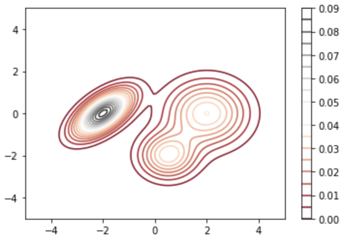 This is the contour map of the 2D distribution that we want to sample from. I created it by mixing 3 normal distributions (Gaussian Mixture Model), and we can get the value of the pdf by calling the following function:
pdf(0,0)
will return 0.0061428136030171505
# create our starting point
x = 0
y = 0
# xVals, yVals will store the coordinates of our samples
xVals = []
yVals = []
for itter in range(10000): # running MH for 10000
    #Sample the proposal distribution which is a standard normal distribution
    xProposed,yProposed = np.random.multivariate_normal([x,y], [[1,0],[0,1]], 1)[0]
    #Calculate the acceptance probability
    AcceptancePrb = min(1,pdf(xProposed,yProposed)/pdf(x,y))
    if(np.random.uniform()<=AcceptancePrb): #Randomly choose whether to keep the proposed sample
        x = xProposed
        y = yProposed
        #Adding our new sample to our sample set
        xVals.append(x)
        yVals.append(y)

    else:
        #Adding our original sample again to the sample set
        xVals.append(x)
        yVals.append(y)
Results
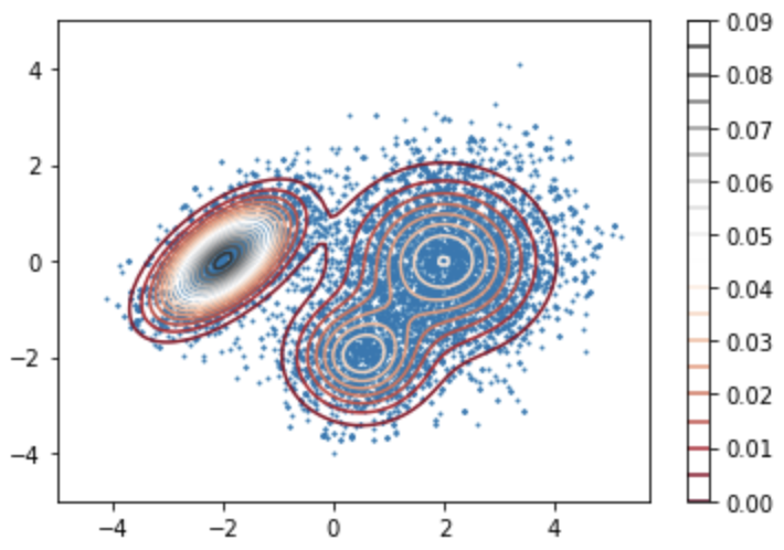 This is the scatter plot for
 xVals, yVals overlayed with the original distribution we wanted to sample from. We can see that it resembles the Gaussian mixture pretty well.