Q Learning

Q Learning is the first Reinforcement Learning technique I learned, its a fun and fundemental and not too difficult to understand.

Overview

I will create a small problem, so that you can see Q Learning in action. So below, we have a small “world”, where we have a beetle that wants to get to a small blueberry (the blue node). This world can be repersented as a directed graph.

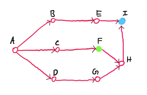
Node A is the starting node, and node I is blueberry node. There are intermediate nodes, and the at node F, there is a bird, one that can eat the beetle. The beetle’s task is to find the most efficient path to the blueberry. We will place a reward of +1 on the blueberry node, and a reward of -1 on the bird node. The goal of Q Learning is to assign a value to each edge, which is equvalent to a state action pair, Q(s,a). The collection of Q(s,a) for all states and their actions is called a Q Table. We initilize the Q Table randomly, after running the Q Learning algorthim, the Q Table should converge such for a given state, the best action will have the highest Q value.

Q Learning algorithm

In Q Learning we move our agent around the world and keep applying the below equation to update the Q Table. For n episodes, we place the agent on a starting node (A in this case) and let the agent move for t itterations. How we let the agent move is nuanced, we will go into that in the epsilon section.
The Q Value update equation is:

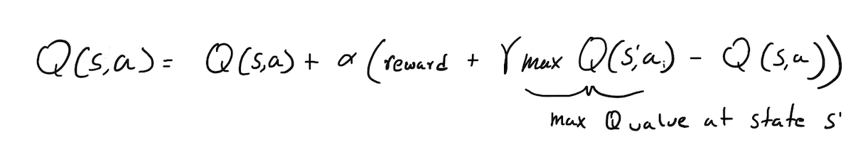
Alpha is the learning rate, and gamma is the discount rate, we will go into those more spefically later. So why does this work, well imagine the edges that connect to the berry, after enough itterations they will have a high Q value, then the edges the connect to that node will have a high Q value, but a lower one since its equal to gamma(max_Q(s’,a). gamma(max_Q(s’,a’) means that if we are at state s’, which is the state the agent moved to from state s then, what is the highest Q value at s’. Gamma, the learning rate controls how much can distant rewards can influence the current Q value, values closer to 1 will produce an agent that is more sensitive for distant rewards and vice versa (Wikipedia). Alpha, controls how senstive the agent is to new information (Wikipedia). So what is the intution behind this algorithm? The edges that connect to the evil bird node, will have a negative Q value, since it has a negative reward, and consequently the edges that those edes that connect to the bird node will also have a negative but of smaller magnitude Q value due to gamma.

Epsilon

Now a imporant part of the algorithm is how should we let the agent move. If look at this problem in general, we would want the agent to move randomly, since our inital Q values are nonsense (they are random), thus we don’t want the agent to strictly follow it. Therefore, at first we would want our agent to move completly randomly, and as our Q values actually become useful, in that we hopefully have some idea of where rewards are, then we want to search those paths more often, eventually to the point where the Q values converege. Thus, as we go through the episodes, we want to follow the Q values more and move randomly less. So how do we implement this, well thats what epsilon is all about. We set epsilon = 1 at first, then we move randomly if np.random.rand() < epsilon. To lower epsilon, we multiply it by the hyperparameter: epsilonDecay = .99. Thus after 100 episodes, epsilon will equal 0.366, in practice we want this lower but since our world is very simple in that most nodes have only 1 possible action, it doesn’t really matter in our case.

Results

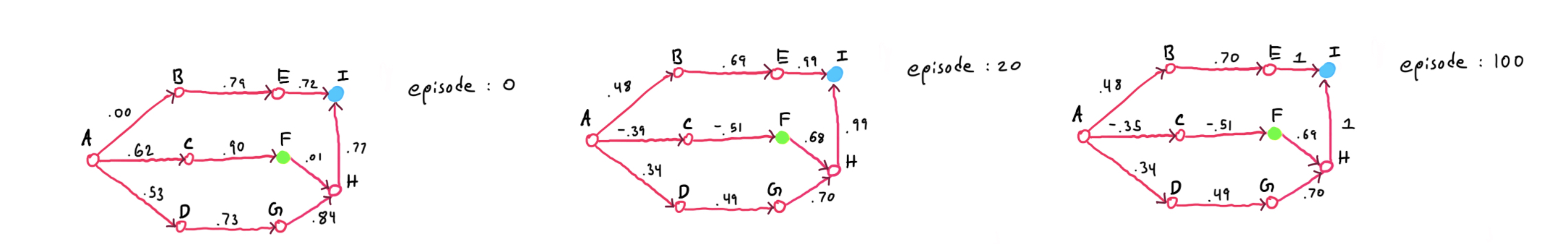
I wrote a python program to actually compute the Q values, and given enough episodes (each itteration), the Q values will converge, which they do. Here is 5 stages of our world and its Q values, for the itterations 0,20,100. I skipped 40,60,80 since they were almost idenitical to 100. As you can see our beetle has learned a good set of Q values to guide it to the berry in the most efficient (shortest) and safest manner. The code that produced this is at the bottom.

Code

import numpy as np
import random

def genQTable(graph):
	QTable = {}
	for node1 in graph:
		for node2 in graph[node1]:
			if(((node1,node2) in QTable) == False):
				QTable[(node1,node2)] = np.random.rand()
	return(QTable)
			
def maxMove(QTable, current):
	if(current == 'I'):
		return(0,0)
	bestNode = graph[current][0]
	for node in graph[current]:
		if(QTable[(current,node)] > QTable[(current,bestNode)]):
			bestNode = node
	return(bestNode, QTable[(current,bestNode)])


def reward(node):
	if(node == 'I'):
		return(1)
	if(node == 'F'):
		return(-1)
	return(0)

graph = {'A':['B','C','D'],
		 'B':['E'],
		 'C':['F'],
		 'D':['G'],
		 'E':['I'],
		 'F':['H'],
		 'H':['I'],
		 'G':['H']}

QTable = genQTable(graph)

# These hyperparameters are not the norm, I was just experimenting. 
startNode = "A"
endNode = "I"
episodes = 100
episodeLength = 10
epsilon = 1
epsilonDecay = .99
gamma = .7
alpha = .7

for episode in range(episodes):
	current = startNode
	if(episode % 20 == 0):
		print(QTable, "episode: ", episode)
	for itteration in range(episodeLength):
		if(np.random.rand() < epsilon):
			prev = current
			current = random.choice(graph[current])
		else:
			prev = current
			current = maxMove(QTable, current)[0]
		QTable[(prev,current)] = QTable[(prev,current)] + alpha*(reward(current) + gamma*maxMove(QTable, current)[1]-QTable[(prev,current)])

		if(current == endNode):
			break
	epsilon *= epsilonDecay

print(QTable)

My next post will be of policy gradients, stay tuned for that!