Variational Autoencoders (VAE)

Introduction

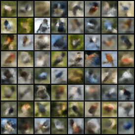
Variational autoencoders merge deep learning and probability in a very intriguing way. If you have heard of autoencoders, variational autoencoders are similar but are much better for generating data. Many resources explain why vanilla autoencoders aren’t good generative models, but the gist is that the latent space is not compact, and there are lots of dead space that produces jargon. We will explain the theory behind VAEs, and implement a model in PyTorch to generate the following images of birds.

Variational Inference (ELBO)

Variational autoencoder takes pillar ideas from variational inference. I will explain what these pillars are. First, there is something called ELBO. Let me plop down a derivation and a graphical model that we are going to work with, it is ubiquitous, so you probably have seen this.
The graphical model:

The equations:

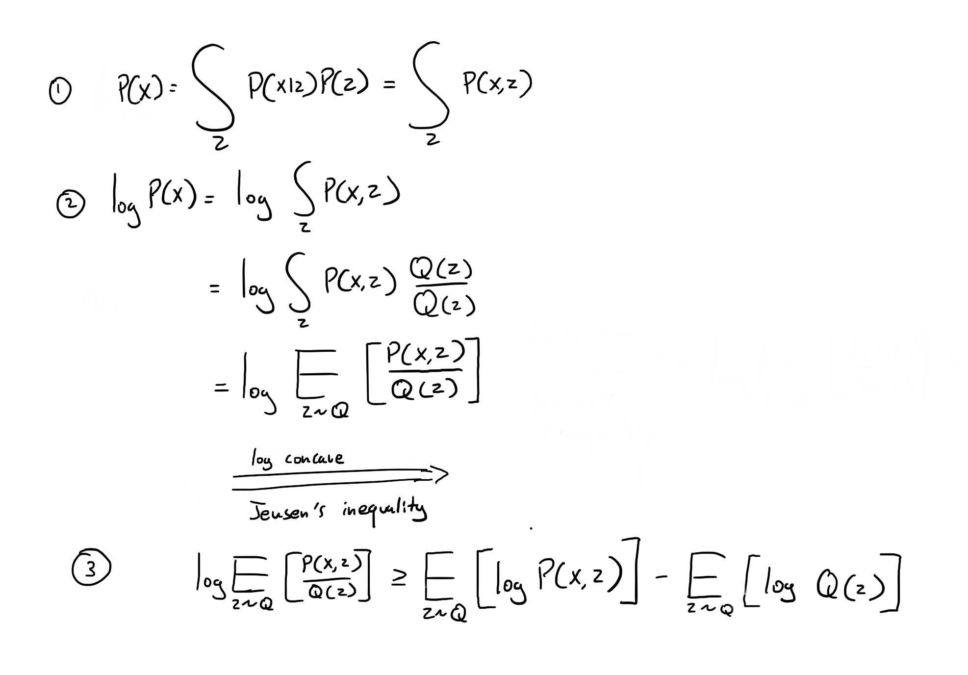
The first key step is how do we go from equation 2 to 3, and that is done by Jensen’s inequality which recognizes that the logarithmic function is concave. Equation 3 is the lower bound of the log P(x), so maximizing this lower bound is going to push log P(x) up.

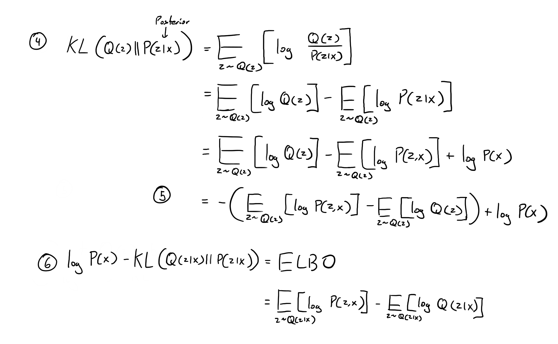
Then we start with the definition of KL divergence (Kullback Leiber Divergence) at step 4. We want to find how close a distribution Q(z) is to the posterior P(z|x). After a series of manipulations, we reach step 5. We can see that the KL divergence between Q(z) and P(z|x) is equal to -ELBO + log P(X). If we are interested in changing Q(z) to be as close as possible as P(z|x), then we want to maximize ELBO since log P(x) does not depend on Q(z).

Taking a closer look at Q(z), we see that if we want to minimize KL(Q(z)||P(z|x)), what we are doing is saying for a given x are fitting Q(z) to its posterior. In our dataset, we are going to many many different x, so having one distribution Q(z) isn’t going to perform well for the posterior. Instead, let’s make Q(z) be a conditional distribution on x, so for a given x it will be the specific posterior for that x, thus instead of Q(z) we have Q(z|x). Now equation 6 should make sense.

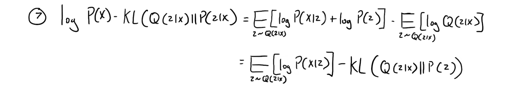
After substituting P(x|z)P(z) for P(z,x) and moving P(z) to the second expectation since they are both from the same expectation distribution where z ~ Q(z|x), we arrive at equation 7.

Constructing A Model

Variational Autoencoders are based on equation 7. So let’s see how we can go from equation 7 to a model that is representative of it. Starting with the left hand side, we have log P(X) - KL(Q(z|x)||P(z|x)). If we want our model to produce good values of x, then the left-hand size should be maximized. Therefore, we should maximize the left-hand side. The first term, E [log P(x|z)] says whats the expected value of log P(x|z) if z is coming from Q(z|x). Therefore we can think of this as the oppo reconstruction error. Meaning, say x is an image of a bird, then if my model is good where Q(z|x) can produce the ideal conditional distribution that can be used to generate that image of the bird then, then that expectation should be high. Moving onto the second term which is -KL(Q(z|x)||P(z)), if we have to maximize the whole right side, then this term should me maximized, so the KL term should me minimized. Now here is where we do some engineering. We want this KL divergence to be tractable. If both Q(z|x) and P(z) are Gaussians, then there is a closed-form solution. We set P(z) to be the unit gaussian, so this will force Q(z|x) to be regions within it, it can’t be full unit gaussian because then it won’t produce a specific distribution for z, and we won’t get a good reconstruction. < br />

Now let’s define our distributions, and how we can model them. For Q(z|x) we will use a neural network that produces the parameters for the gaussian for an inputted x. Then we will use those parameters to sample a z which is the input for another neural network which is our P(x|z), and that network will try to replicate the original x. Then we can define our loss to be the reconstruction loss as well as the KL divergence between Q(z|x) and the unit gaussian.

This is the model we have now

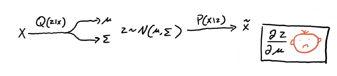
Reparameterization

There is an issue with the above model, hence the sad face. If we are going to use gradient descent, our whole model should be differentiable, such that we can find the partial derivative for each parameter. However, if we try to find the partial derivative for the encoder’s parameters, we would be unsuccessful due to the sampling. We need to work around the sampling, such that the gradients can “flow”. This is where the reparameterization comes in. Observe the updated model below.

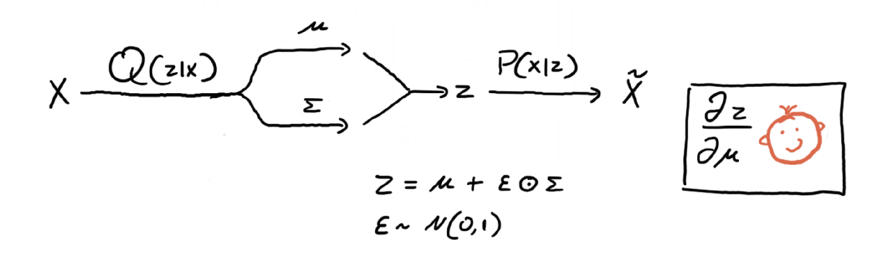
Here we introduced a new variable, that sampled from a normal gaussian of the same number of dimensions as Q(z|x). We are replicating the same sampling process from the original model, except now we can compute the partial derivative of z with respect to mu or sigma, thus our model is fully differentiable. So we can use gradient descent, hence the happy face.

That’s it! Now we keep taking some images from our dataset and training the model. Once the model is trained, it will be able to reproduce the original image (hopefully).

Implementation

I wrote the following implementation, which uses convolutional layers and transposed convolutional layers instead of normal dense layers since we are dealing with images. I am certain that if you tinker around or have better domain knowledge, you can come up with a more efficient architecture.

import matplotlib.pyplot as plt
import matplotlib
import torch
from torchvision import datasets, transforms
import torchvision
from PIL import Image
import numpy as np
import torch.nn as nn
import torch.nn.functional as F
import torch.optim as optim

matplotlib.use('TkAgg')
device = torch.device("cuda:0" if torch.cuda.is_available() else "cpu")
print(device)

transform = transforms.Compose([transforms.ToTensor(),transforms.Resize((32,32))])
dataset = datasets.ImageFolder("images", transform)
dataloader = torch.utils.data.DataLoader(dataset, batch_size=32, shuffle=True)
images, labels = next(iter(dataloader))

def imsave(name,img):
	npimg = img.numpy()
	plt.imsave(name,np.transpose(npimg, (1, 2, 0)))

#imshow(torchvision.utils.make_grid(images))

class VAE(nn.Module):
	def __init__(self):
		super(VAE, self).__init__()
		self.eConv1 = nn.Conv2d(3,6,4)
		self.eConv2 = nn.Conv2d(6,12,5)
		self.ePool1 = nn.MaxPool2d(2,2)
		self.eConv3 = nn.Conv2d(12,24,5)
		self.ePool2 = nn.MaxPool2d(2,2)
		self.eF1 = nn.Linear(24*4*4,180)
		self.eMu = nn.Linear(180,180)
		self.eSigma = nn.Linear(180,180)

		self.dConvT1 = nn.ConvTranspose2d(180,200,4)
		self.dBatchNorm1 = nn.BatchNorm2d(200)
		self.dConvT2 = nn.ConvTranspose2d(200,120,6,2)
		self.dBatchNorm2 = nn.BatchNorm2d(120)
		self.dConvT3 = nn.ConvTranspose2d(120,60,6,2)
		self.dBatchNorm3 = nn.BatchNorm2d(60)
		self.dConvT4 = nn.ConvTranspose2d(60,3,5,1)

	def encode(self,x):
		x = self.eConv1(x)
		x = F.relu(x)
		x = self.eConv2(x)
		x = F.relu(x)
		x = self.ePool1(x)
		x = self.eConv3(x)
		x = F.relu(x)
		x = self.ePool2(x)
		x = x.view(x.size()[0], -1)
		x = self.eF1(x)
		mu = self.eMu(x)
		sigma = self.eSigma(x)
		return((mu,sigma))

	# From https://github.com/pytorch/examples/blob/master/vae/main.py
	def reparameterize(self,mu,sigma):
		std = torch.exp(0.5*sigma)
		eps = torch.randn_like(std)
		return (mu + eps*std)

	def decode(self,x):
		x = torch.reshape(x,(x.shape[0],180,1,1))
		x = self.dConvT1(x)
		x = self.dBatchNorm1(x)
		x = F.relu(x)
		x = self.dConvT2(x)
		x = self.dBatchNorm2(x)
		x = F.relu(x)
		x = self.dConvT3(x)
		x = self.dBatchNorm3(x)
		x = F.relu(x)
		x = self.dConvT4(x)
		x = torch.sigmoid(x)
		return(x)
		
	def forward(self,x):
		mu,sigma = self.encode(x)
		z = self.reparameterize(mu,sigma)
		x_gen = self.decode(z)
		return((x_gen,mu,sigma))
		
# From https://github.com/pytorch/examples/blob/master/vae/main.py
# Reconstruction + KL divergence losses summed over all elements and batch
def loss_function(x, x_gen, mu, sigma):
	#print(x.shape)
	#print(x_gen.shape)
	BCE = F.binary_cross_entropy(x_gen, x, reduction='sum')

	# see Appendix B from VAE paper:
	# Kingma and Welling. Auto-Encoding Variational Bayes. ICLR, 2014
	# https://arxiv.org/abs/1312.6114
	# 0.5 * sum(1 + log(sigma^2) - mu^2 - sigma^2)
	KLD = -0.5 * torch.sum(1 + sigma - mu.pow(2) - sigma.exp())

	return BCE + KLD

vae = VAE()
vae.to(device)

optimizer = optim.Adam(vae.parameters(), lr=1e-3)

for epoch in range(200):

	running_loss = 0.0
	for i, data in enumerate(dataloader, 0):
		# get the inputs; data is a list of [inputs, labels]
		images = data[0].to(device)
		#images = data[0]
		# zero the parameter gradients
		optimizer.zero_grad()

		# forward + backward + optimize
		outputs = vae(images)
		loss = loss_function(images, outputs[0], outputs[1], outputs[2])
		loss.backward()
		optimizer.step()

		# print statistics
		running_loss += loss.item()
		if i % 500 == 499:    # print every 500 mini-batches
			print('[%d, %5d] loss: %.3f' %
				  (epoch + 1, i + 1, running_loss / 2000))
			running_loss = 0.0

	PATH = 'vae_checkpoints/'
	torch.save(vae.state_dict(), PATH+str(epoch)+".pt")
	imsave("actual/" + str(epoch) + ".png", torchvision.utils.make_grid(images.cpu()))
	imsave("recon/" + str(epoch) + ".png",torchvision.utils.make_grid(outputs[0].detach().cpu()))

print('Finished Training')

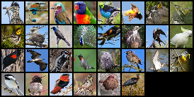
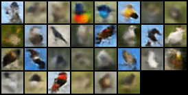
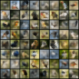
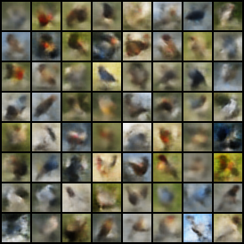
This model was trained on Caltech-UCSD Birds 200. Below to the left is a real batch of images from the dataset, and the right image is the ouput of the model.

Generation

I said that VAEs are generative models, so it lets generate some birds! All I do is sample many z from the unit gaussian P(Z), and volia.

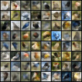
Here is the code that I wrote to generate the images.

import matplotlib.pyplot as plt
import matplotlib
import torch
from torchvision import datasets, transforms
import torchvision
from PIL import Image
import numpy as np
import torch.nn as nn
import torch.nn.functional as F
import torch.optim as optim

def imsave(name,img):
	npimg = img.numpy()
	plt.imsave(name,np.transpose(npimg, (1, 2, 0)))

class VAE(nn.Module):
	def __init__(self):
		super(VAE, self).__init__()
		self.eConv1 = nn.Conv2d(3,6,4)
		self.eConv2 = nn.Conv2d(6,12,5)
		self.ePool1 = nn.MaxPool2d(2,2)
		self.eConv3 = nn.Conv2d(12,24,5)
		self.ePool2 = nn.MaxPool2d(2,2)
		self.eF1 = nn.Linear(24*4*4,180)
		self.eMu = nn.Linear(180,180)
		self.eSigma = nn.Linear(180,180)

		self.dConvT1 = nn.ConvTranspose2d(180,200,4)
		self.dBatchNorm1 = nn.BatchNorm2d(200)
		self.dConvT2 = nn.ConvTranspose2d(200,120,6,2)
		self.dBatchNorm2 = nn.BatchNorm2d(120)
		self.dConvT3 = nn.ConvTranspose2d(120,60,6,2)
		self.dBatchNorm3 = nn.BatchNorm2d(60)
		self.dConvT4 = nn.ConvTranspose2d(60,3,5,1)

	def encode(self,x):
		x = self.eConv1(x)
		x = F.relu(x)
		x = self.eConv2(x)
		x = F.relu(x)
		x = self.ePool1(x)
		x = self.eConv3(x)
		x = F.relu(x)
		x = self.ePool2(x)
		x = x.view(x.size()[0], -1)
		x = self.eF1(x)
		mu = self.eMu(x)
		sigma = self.eSigma(x)
		return((mu,sigma))

	# From Documentation
	def reparameterize(self,mu,sigma):
		std = torch.exp(0.5*sigma)
		eps = torch.randn_like(std)
		return (mu + eps*std)

	def decode(self,x):
		x = torch.reshape(x,(x.shape[0],180,1,1))
		x = self.dConvT1(x)
		x = self.dBatchNorm1(x)
		x = F.relu(x)
		x = self.dConvT2(x)
		x = self.dBatchNorm2(x)
		x = F.relu(x)
		x = self.dConvT3(x)
		x = self.dBatchNorm3(x)
		x = F.relu(x)
		x = self.dConvT4(x)
		x = torch.sigmoid(x)
		return(x)
		
	def forward(self,x):
		mu,sigma = self.encode(x)
		z = self.reparameterize(mu,sigma)
		x_gen = self.decode(z)
		return((x_gen,mu,sigma))

vae = VAE()
vae.load_state_dict(torch.load("vae_checkpoints/198.pt"))
vae.eval()

vectors = torch.randn(64, 180, 1, 1)
images = vae.decode(vectors)
imsave("grid3.png", torchvision.utils.make_grid(images.detach()))