Improving Recurrent Models with Group Theory

Today’s article is going to be about understanding combination of the following papers: Unlocking State-Tracking in Linear RNNS Through Negative Eigenvalues, DeltaProduct: Increasing the Expressivity of DeltaNet Through Products of Householders by Riccardo Grazzi and Julien Siems and others. I came across this paper through the ASAP Seminar.

Motivation: First to put down some notation, we will denote a recurrent model as

In the DeltaNet formulation, $A(x_t) = I - \beta_t k_t k_t^\top, \,\,\,B(x_t) = \beta_tk_tv_t^\top, \text{dec}(H_t, x_t) = H_t^\top q_t$

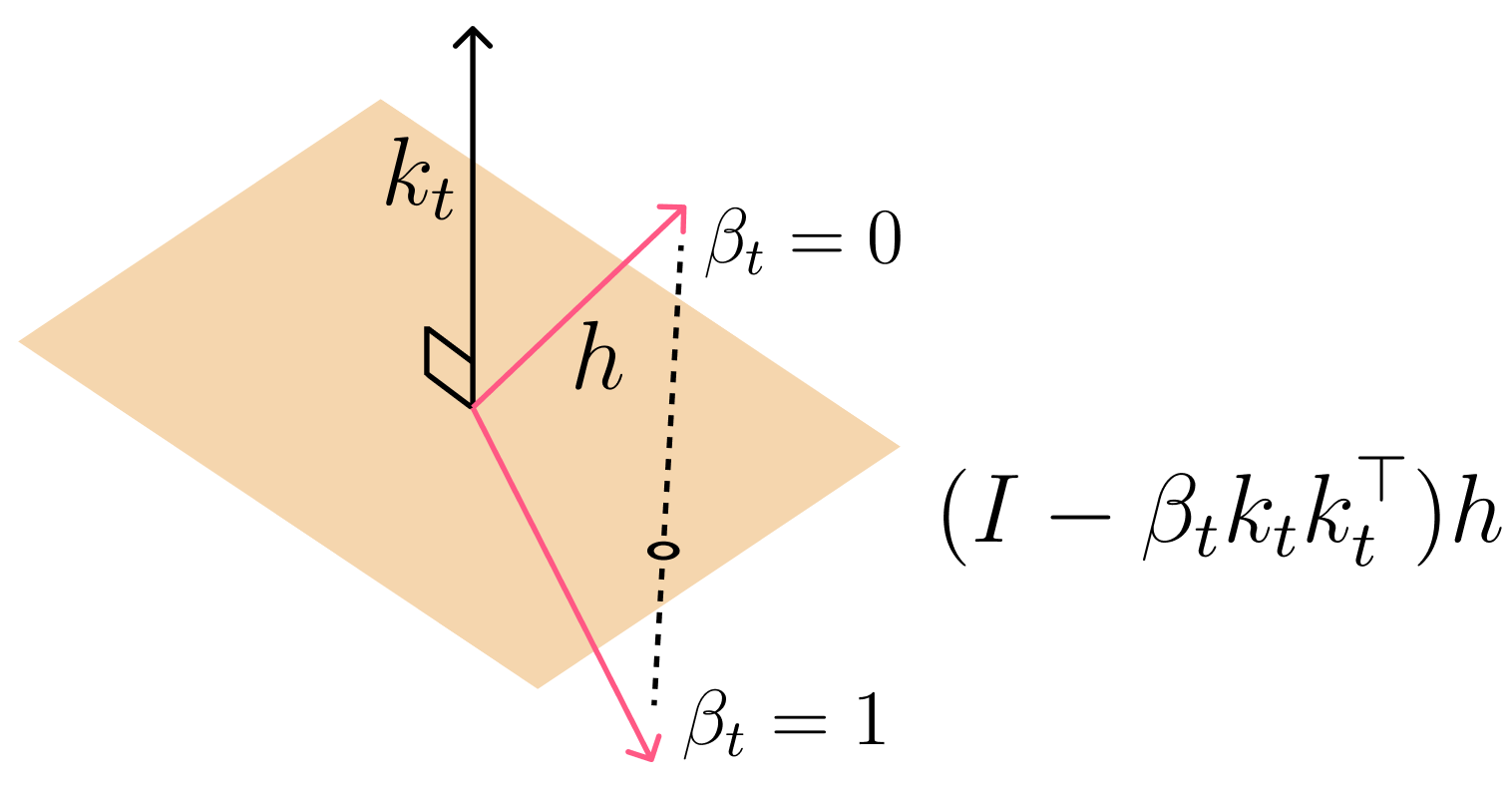
This can also be seen as 1 step gradient descent on $\frac{1}{2}\lVert H^\top k_t - v_t \rVert^\text{2}_\text{2}$. Importantly, since $\lVert k_t \rVert = 1$ and the range of $\beta_t \in [0,1]$, and this means the eigen values of $A(x_t)$ are bounded between $[0,1]$. Therefore, if we modify the update to be $A(x_t) = I - \text{2}\beta_t k_t k_t^\top$, then this makes the eigenvalues be in the range $[-1,1]$. Interestingly, this is a householder matrix! To refresh our memory house holder transformations are reflections.

In this article, we focus on how a particular extension enables recurrent models to solve state tracking problems, especially those that arise in structured domains like group theory. To set the stage, recall that a group is a set equipped with an operation that satisfies four key properties: closure, associativity, the existence of an identity element, and the existence of inverses. A powerful result in abstract algebra is Cayley’s theorem, which states that every finite group is isomorphic to a subgroup of the symmetric group $S_n$, the group of all permutations of $n$ elements. This means that, in principle, any finite group computation can be modeled using permutations.

One state tracking problem we consider involves the symmetric group $S_n$. The input is a sequence of permutations $x_1,x_2, \dots ,x_t$ and the goal is for the model to output the cumulative group element at each step:

where $\cdot$ denotes composition of permutations, and the product is taken from right to left (i.e., $x_1$ is applied first). This task requires the model to maintain a hidden state that effectively encodes the current group element, updating it with each new permutation.

As a concrete example, let $x_1=(1,2)(3,4)$ and $x_2=(1,3)(2,4)$, both elements of $S_4$. Then the desired output after the second step is $y_2=x_2 \cdot x_1=(1,4)(2,3)$, which is the result of composing the two permutations.

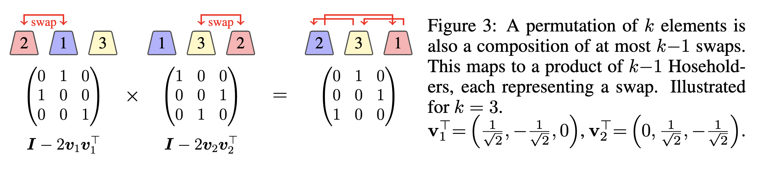
So how does this relate to Householder transformations? When permutations are viewed as transformations acting on a space, swaps can be naturally expressed using Householder reflections—a class of orthogonal transformations that reflect vectors across hyperplanes. This connection allows us to embed group operations directly into the linear dynamics of recurrent models, facilitating state tracking. The paper provides a helpful figure that visually demonstrates how permutations correspond to sequences of Householder reflections.

This also implies that if I am operating on $S_n$, then I would need $n-1$ householder reflections. And this brings us to the DeltaProduct Formulation: For each token $x_i$, generate $n_h$ keys, values, and step sizes (the betas):

where:

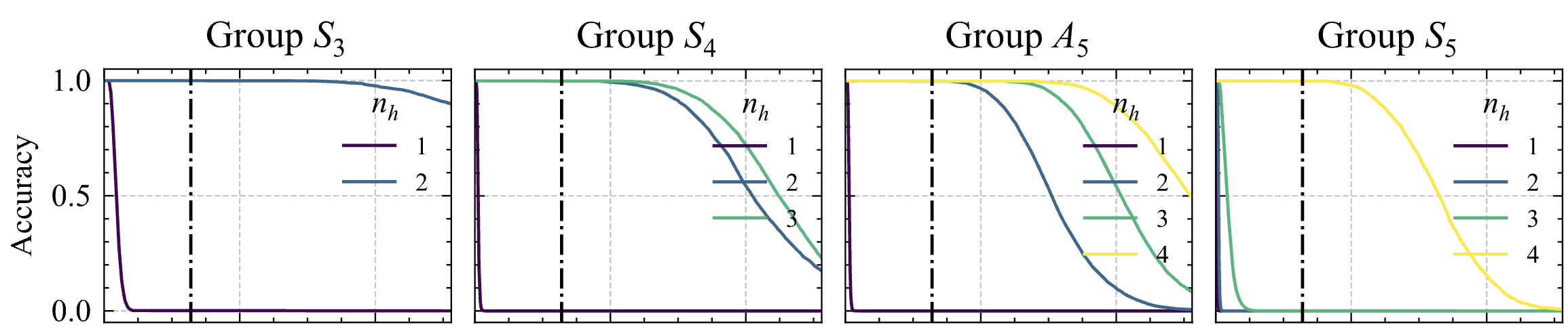
So to put in words, we are expanding our hidden state update to do $n_h$ updates, each step having its own dedicated weight to produce a house holder transformation. This can also be seen as doing $n_h$ steps of gradient descent on the associate recall objective. Now this will allow us to perform state tracking. Interestingly, there is a case where in $S_4, A_5$ you only need $n_h=2$, instead of the theoretical value 3. See the following Figure 3.

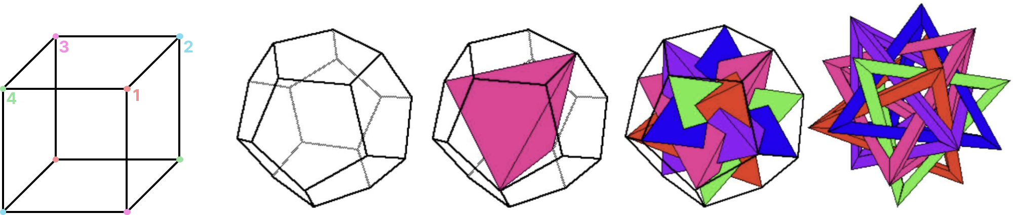
The reason is they are isomorphic to subgroups of $\text{SO}(3, \mathbb{R})$. To see this, first consider the $S_4$ setting where we have an ordering of 4 elements. Interestingly, we can represent these 4 elements as the diagonals of a 3D cube. The operations on this cube are orientation preserving rotations, and you can record the ordering of the 4 diagonals post transformation as the new group element. Now, things for $A_5$ are a bit more involved. $A_5$ is the alternating group of 5 elements, the alternating group has only even permutations of the 5 elements - meaning there are an even number of swaps to create the permutations. We can actually treat each element as the position of a colored tetrahedron inside an icosahedron, and again we can rotate the icosahedron while preserving its orientation and record the position of the tetrahedrons after a rotation. See both examples below, and the icosahedron is taken from this article.

In addition, the Cartan-Dieudonné theorem, states that

that every orthogonal transformation in an n-dimensional symmetric bilinear space can be described as the composition of at most n reflections.

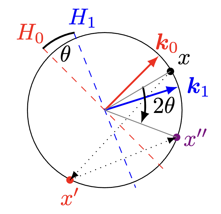
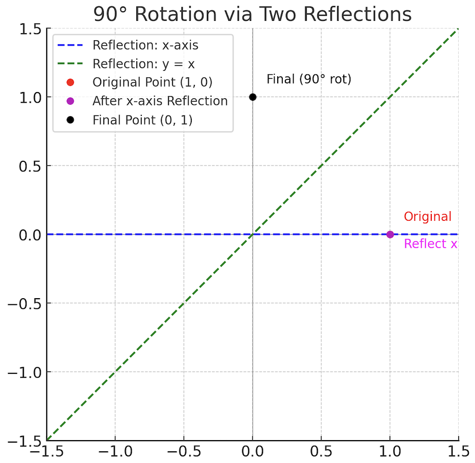
For a rotation in 3D space, we just need 2 reflections, provided that our keys are also in subspace of dimension 3. This explains why $n_h$ can be just 2. Here are some illustrations to explain this geometrically. The first one is from the paper, and the second was generated in Matplotlib just for myself to see an example.

Acknowledgement

Big thanks to Riccardo Grazzi, and Julien Siems for reading the article and providing really helpful feedback on adding more depth.

References:

https://en.wikipedia.org/wiki/Householder_transformation

https://en.wikipedia.org/wiki/Cartan–Dieudonné_theorem

https://en.wikipedia.org/wiki/Symmetric_group

https://arxiv.org/abs/2404.08819

https://en.wikipedia.org/wiki/Alternating_group