MoE

Introduction

Mixture of Experts (MoE) have gotten popular recently with the rise of large language models and multi modal reasoning. They are not a new idea, and have existed for a while in the form of Ensemble Methods. For example, you might have heard of Bagging and Boosting. Bagging refers to training different models on different random partitions of data and then aggregate their results to produce a more robust model. Boosting involves training models sequentially, and each consecutive model is trained on a reweighed data depending on the previous models performance. In addition, you probably have seen models like Gaussian Mixture Models. While they are simple, they capture the essence of the motivation for a mixture model, model a more complex distribution through explicit use of simple distributions / functions.

Key Papers

To be transparent, most of the papers I choose are the ones that Finbarr Timbers used it his awesome blogs on MoE, make sure to check his page out! He seemed to already capture the key ideas, but hopefully I added some extra insights.

OUTRAGEOUSLY LARGE NEURAL NETWORKS:
THE SPARSELY-GATED MIXTURE-OF-EXPERTS LAYER

They present a model in the form

Both $W_g, W_{\text{noise}}$ are learned through normal back propogation. I think a important takeaway is the $W_{\text{noise}}$ parameters, because it allows for exploration, but under expectation, once $E_i(x)$ converge to their optimal functions, then $W_\text{noise}$ should converge to zero as $Wg_i$ converges to the optimal value. In addition $k$ should be larger than one, because the SwitchFormer authors write that

Shazeer et al. (2017) conjectured that routing to k > 1 experts was necessary in order to have non-trivial gradients to the routing functions. The authors intuited that learning to route would not work without the ability to compare at least two experts.

The authors convey that problem that often arises in these setups is

We have observed that the gating network tends to converge to a state where it always produces large weights for the same few experts. This imbalance is self-reinforcing, as the favored experts are trained more rapidly and thus are selected even more by the gating network. Eigen et al. (2013) describe the same phenomenon, and use a hard constraint at the beginning of training to avoid this local minimum. Bengio et al. (2015) include a soft constraint on the batch-wise average of each gate.

To mitigate this issue, they introduce a Importance loss term that tries to enforce a higher variation of the gating value over a batch $X$.

Where CV is the coefficient of variation $\sigma/\mu$. This encourages the model to have uniform gating across a batch. However, is still not computationally ideal because of the following reason.

The authors write that

We want to define an additional loss function to encourage experts to receive roughly equal numbers of training examples. Unfortunately, the number of examples received by an expert is a discrete quantity, so it can not be used in backpropagation.

This also helps in a distributed setup, where computationally is more evenly spread across.

The problem with the $\text{Importance}$ loss term is that, as you sum across the batch you loose information of the gate values for individual data points in the batch, this information loss is why the aforementioned problem arises. So the authors have a new metric

Let $P(x,i)$ denote the probability that “probability that $G(x)_i$ is nonzero, given a new random choice of noise on element $i$, but keeping the already-sampled choices of noise on the other elements”. And they create an additional loss term which will spread apart values per each column which will prevent the degenerate case that the Importance term can suffer from.

Something I am not sure about is why we can’t just use the Load loss term and drop the Importance term. One final detail is they set $W_{\text{noise}}, W_g$ to all zeros because that will have a uniform weighting over the experts initially, which helps with allowing them to specialize.

Switch Transformers: Scaling to Trillion Parameter Models
with Simple and Efficient Sparsity

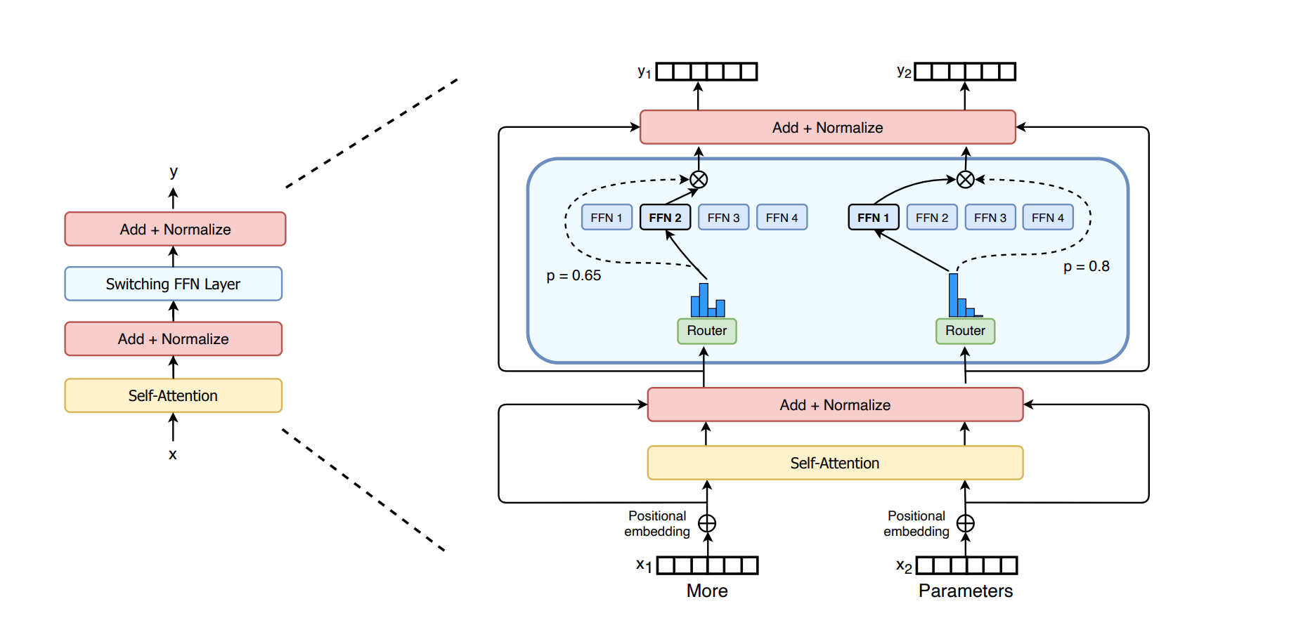
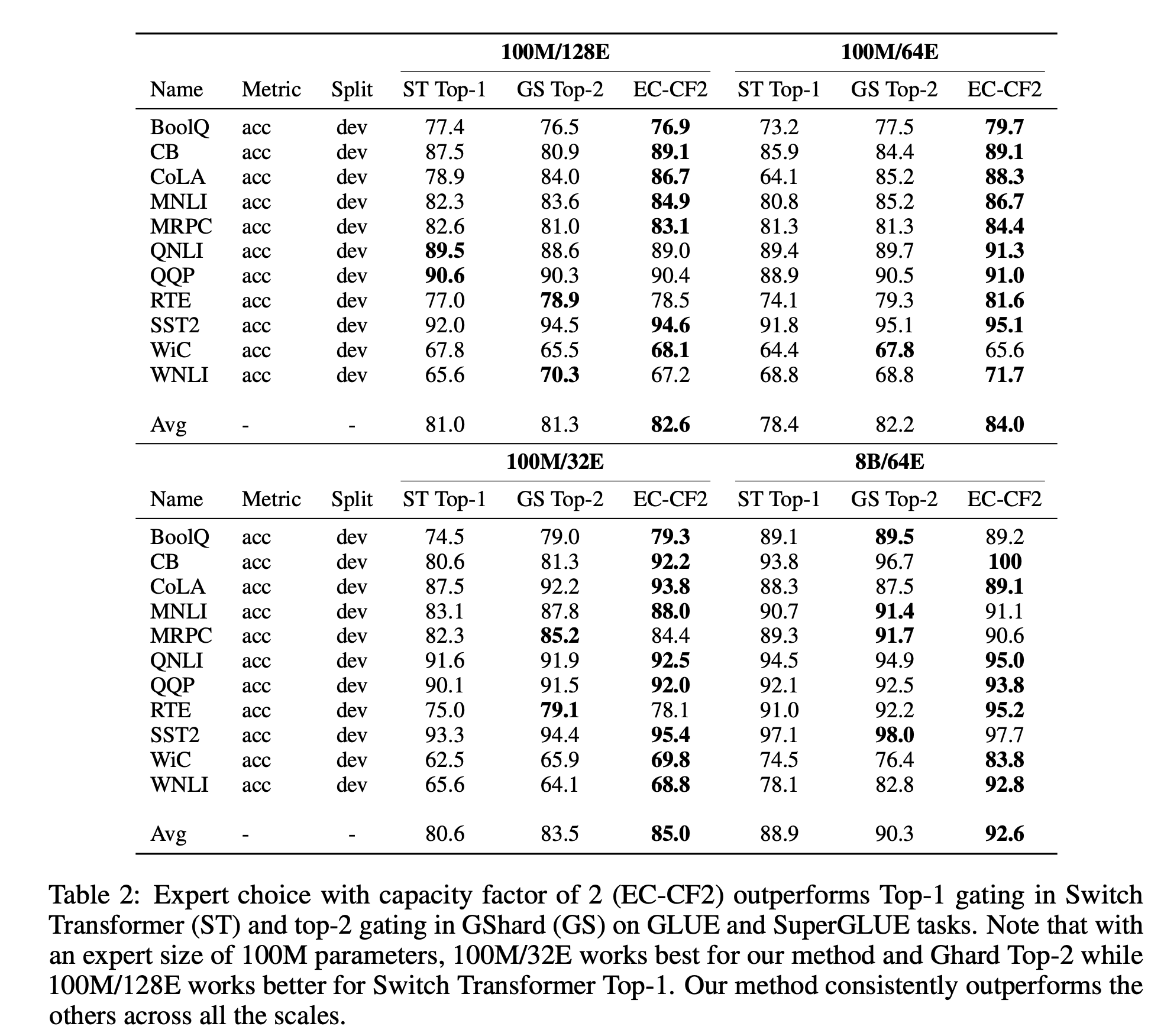
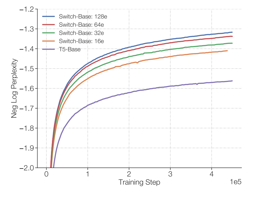
Each token is routed to one expert. So this different than previous works that show that tokens should be routed for multiple experts. The authors show that this is no longer the case and this also improves computational efficiency.

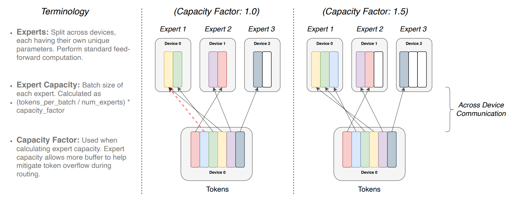
In this figure we see that for a batch of tokens, each expert has a budget of how many tokens they can process in total. This is denoted by the Expert Capacity. If its too small, then some tokens won’t be processed (the blue one in the left picture), however, too large of a capacity is also inefficient.

For their load balancing loss, let
$N$ be the number of experts, and $B$ be the batch that has $T$ tokens. The loss is:

One neat thing is with this loss, you don’t need to have both a load balancing and importance loss as the previous paper had. Lets unpack what this loss is doing. Since $f_i$ will roughly be aligned with $P_i$ then we can say in a handy wavy way that the loss can be minimized when both are uniform. This also prevents cases where $p_i(x)$ is very unimodal because for the same vector $F = \{f\}_i^N$, there can be mutiple $p_{1-n}(x)$, so the uniform $p$ would minmize the loss the most.

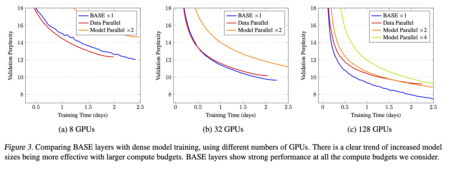
Importantly, the authors show that there is consistently an improvement when adding more experts and this is done with the same computational budget, see figure to the right. And they also show the scaling is better than the traditional dense scaling. See figure below.

Hash Layers For Large Sparse Models

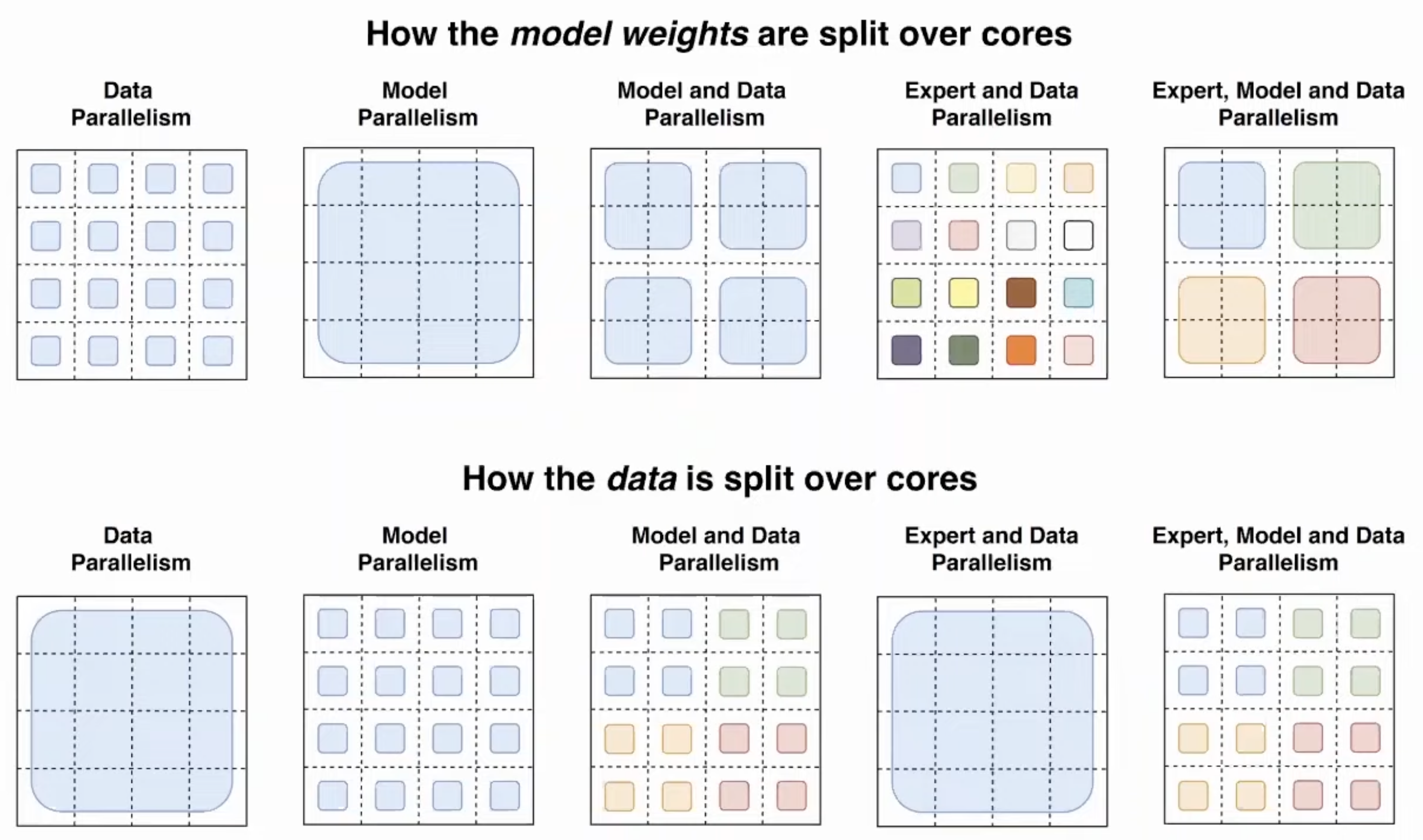
The MoE layers are implemented to replace the feed forward networks in original transformer, SwitchFormer style. Most papers replace the FFN with the MoE layers because FFNs are ‘’the most computationally expensive part in a Transformer-based network” - (Zhou et al. 2022).

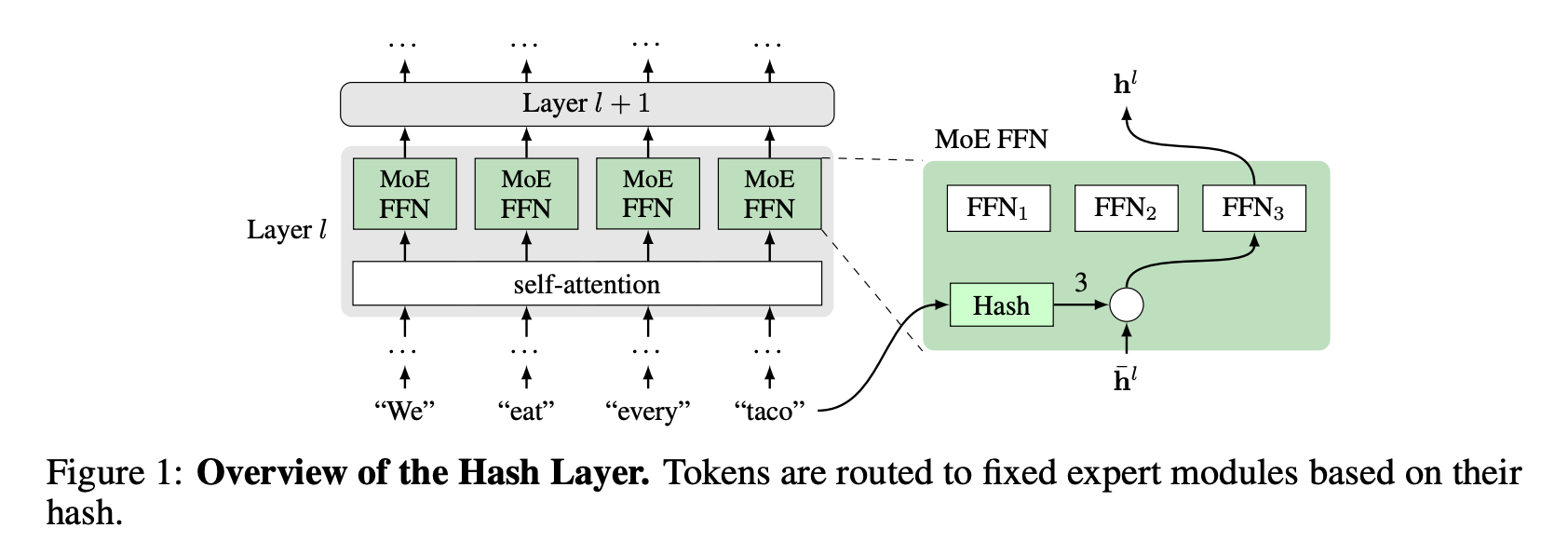
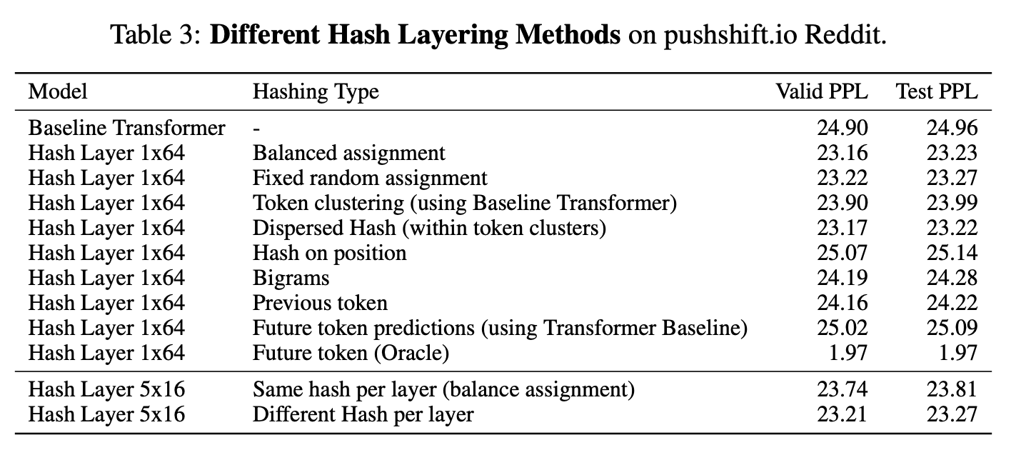
I found this paper pretty surprising because you can get good performance with a random mapping between the token and which FFN it gets routed to. This seems counter intuitive because one would expect that a dynamic routing model that is able to decide which expert to send the token to depending on the token’s embedding would provide for more flexibility. The authors write:

We are free to choose from various possible hash functions, which we will consider below. However, for training purposes, the hash function is fixed in advance, and in this way, our routing mechanism requires no training and has no adjustable parameters …

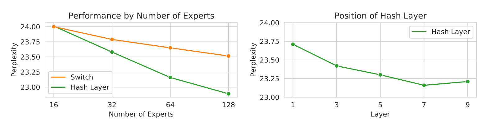
So one problem with this is, because of the Zipfain distribution, which well models the distributions of word frequencies, the distribution of experts being used will also be skewed. So they came up with a
Balanced Hash, which uses the distribution of the training data and tries to rehash to obtain a less skewed distribution over the hash buckets. Another version is the Clustered Hash, which performs k-means on the token embeddings, this will hash similar tokens to the same function. Interestingly they also try the opposite of this where within a cluster from k-means, they will spread out the tokens within that cluster over the buckets. The authors motivation for this is:

very similar tokens need fine distinctions which requires more model capacity (hence assigning to different experts)

One final version they try is to hash part of the weight matrix for the feed forward network: $B(\text{relu}(A(h)))$.

Where, $k_i$ is determined by the hash: $k_i = \text{hash}_i(x)$

DSelect-k: Differentiable Selection in the Mixture of Experts with Applications to Multi-Task Learning

So in most of the other works in this page we often use a top k select over the gating values. The authors of this paper propose that that could lead to instabilities during training, because the loss landscape is no longer smooth. So to reiterate, the prior MoE models often are equivalent to solving:

So here the $L_0$ norm constraint is what makes it difficult for our usual gradient based optimizers. Consequently, the contribution of this work is to convert this into a unconstrained optimization problem. Pretty cool!

This formula can map binary numbers to one hot vectors. For example, if $z = [1,0]$, then $r(z)_2 = 1$, since I am using 0 indexing. Thus we can use this to obtain a mixture over k experts with a stack of k binary numbers which is $Z$.

So our new optimization problem becomes:

But this is still not that useful because $z^{(i)}$ is still a binary vector which becomes a combinatorial optimization problem which is not what we want. So instead lets relax $z^{(i)}$ to be continuous and we can do that with the following.

S(t) smooth function that can exactly equal 0, 1.

The entropy isn’t directly calculated on $Z$ but $\Omega(Z)\coloneqq \sum_{i=1}^kh(r(S(z^{(i)})))$, where $h$ is an entropy function. The authors state that the entropy regularization isn’t needed because empirically the $z^{(i)}$ will become a binary vector, but for faster convergence the entropy term helps. So $\alpha, Z$ does not depend on $x$, but you can easily do that as well via a linear transformation.

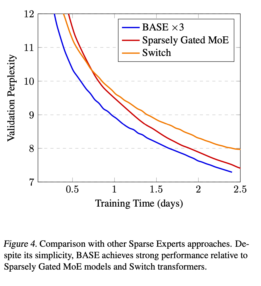
BASE Layers: Simplifying Training of Large, Sparse Models

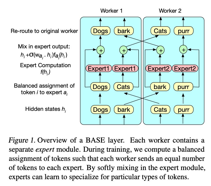
This paper has a similar setup to the previous paper with some key differences. So to go over their notation, they have $E$ experts, and each one is denoted by $f_e$ and its learnable representation $w_e\in \mathbb{R}^D$ to allow us to to routing. $h_t$ is the token embedding and $a_t \in \{0,..., E\}$ is the assignment of the token to expert. So the overall model takes the following form:

The assignment during training and testing is different: the authors write that

During training, we maximize model throughput by assigning an equal number of tokens to each expert. At test time, we simply assign each token to its highest scoring expert.

So during training they solve the well studied assignment problem

Here $T$ is the number of tokens. One potential algorithm to solve this is the famous Hungarian matching one, but that is $O(n^3)$ and not parallelizable. Instead the authors use a different Auction Algorithm (Bertsekas et al. 1922) which is “which is more easily parallelizable on GPUs than the Hungarian Algorithm”.

O
ne important point is that since the partition of the dataset over workers would not be IID, they randomly shuffle the tokens across workers before calculating the assignments.

Mixture-of-Experts with Expert Choice Routing

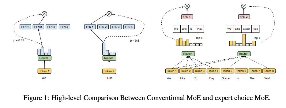
The authors start off by highlighting some of the previous problems with MoE models where the routing function decides which for each token, which expert to route it to. These problems revolve around load imbalance, and as we have seen so far, there are multiple different heuristics / regularizations to encourage more uniform load over the experts. So to be concise, here is how they implement their method:

$X \in \mathbb{R}^{n \times d}$$X \in \mathbb{R}^{n \times d}$$d$$X \in \mathbb{R}^{n \times d}$$d$$X \in \mathbb{R}^{n \times d}$$I$ is an index matrix, and G is the weights of the selection. So then a permutation matrix $P \in \mathbb{R}^{e \times k \times n}$ is calculated based on $I$ to reshuffle the indicies such that $X_{in} \in \mathbb{R}^{e \times k \times d}= PX$ allows you to index the tokens per expert. Then the FFN and reverse shuffle/weighting is defined as:

Notice here that there is nothing to prevent experts taking in the same tokens. While it seems that a more even spread of tokens better utilizes the model’s capacity, they introduce a entropy regularization in the form of:

Where $H(A)$ calculates the entropy. So this is a entropy regularized linear program, and after obtaining $A$, instead of $S^T$ the top k is calculated using $A$. So what this allows is, if $S^T$’s top k are rather skewed towards a small set of tokens, depending on how much larger the top k values are compared to the rest, and $\lambda$, A can reselect a more uniform set of tokens.