Thompson’s Sampling

Imagine you are designing a website that displays news content for a specific user. Specially, on the home page you have 3 options: fill the entire page with science, sports, or political articles. Your objective is to maximize user interaction. Assuming each time a user x interacts with the website is independent of prior interactions, we can model whether the user clicks on one of the presented articles as a Bernoulli random variable.

Over time we want to learn about the user’s interests, and what genre do they like the most so that we can maximize their interaction by presenting news content from that genre. Therefore, we have 3 different Bernoulli random variables at play $X_1, X_2, X_3$: the science RV, sports RV, and Politics RV respectively. Each one is modeled by a parameter $\theta_{i}$, where $i$ is $1,2,3$. Our objective is to design an algorithm that can efficiently learn these parameters $(\theta_{i})$ to determine what is the favorite genre of the user. One classic way is Thompson’s Sampling, and it is heavily based off of some core probability principles which I will go over.

We want to find the expected value of whether the user interacts with a presented genre: to find the ideal one, however $E[X_i] = \theta_i$ and we do not know $\theta_i$. Consequently, we make a random guess about it. Specifically, we establish a prior distribution $P(\theta_i)$. This prior is modeled by the Beta distribution.

With this knowledge it is straight forward to understand Thompson’s Sampling. It first randomly initializes $\alpha_i, \beta_i$ for the priors. Then for each iteration, we sample $\theta_i \sim beta(\alpha_i, \beta_i)$ for $i \in {1,2,3}$. Then based on which $\theta$ is the largest (since $E[X_i] = \theta_i$, we present that genre to the user and set $x$ to be their response (x = 1 if they clicked on one of their articles, and 0 if not). We calculate the posterior $P(\theta_i|x)$ which is just the beta distribution with updated parameters: $beta(\alpha+x, \beta+1-x)$, and we set that distribution as the new prior distribution so now

$P(\theta_i) = beta(\alpha+x, \beta+1-x)$.

Let’s iterate through some scenarios to better understand this algorithm and why its more efficient than a random or greedy search.

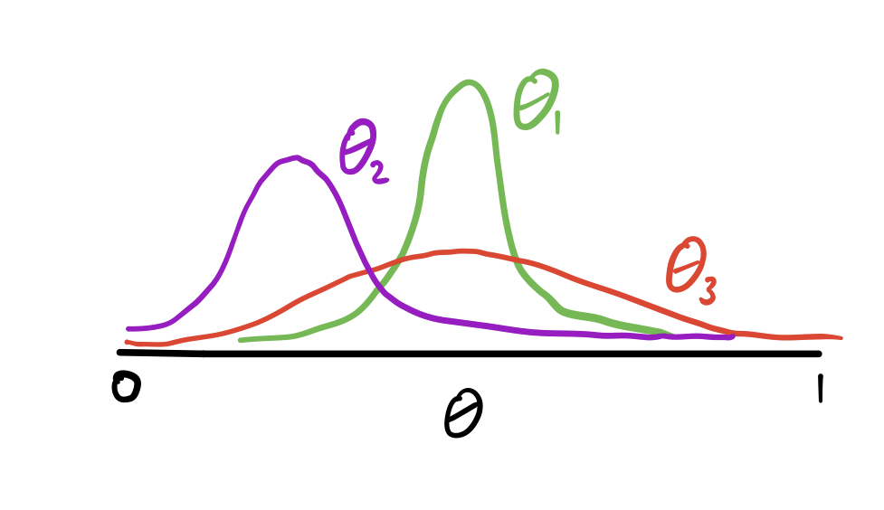
Imagine we are on the $j^{th}$ round, and our priors look like the image above. So if you wanted to have a decent result with high confidence you would pick the green distribution, but we also need to explore because it could be the case the true $\theta_3$ is higher than the true $\theta_2$. We are pretty confident that spending resources to explore $\theta_2$ is not worth it. So how does Thompson’s sampling address these things. First, when we sample an $\theta_i$ from each of the 3 distributions, it is likely that the sampled $\theta_2$ will be lower than $\theta_1$, and thus it will be rarely chosen. However, there is a decent chance that the sampled $\theta_3$ will be larger than the sampled $\theta_1$ and consequently we will spend more time exploring the genre corresponding to the red distribution than the purple one. As we do that we will update our $\alpha, \beta$ parameters and have a better understanding of its distribution.

Eventually if you run Thompson’s sampling enough the distributions should converge to the true distribution of the user’s preferences, especially the best ones. Once we are at this stage, the algorithm naturally will explore less because most of the time the sampled $\theta_i$ from the best genre prior will be the largest.

Here is an implementation of Thompson’s Sampling. In this example we set the user’s preferences to click on science articles .7 of the time, sports .5 of the time, and politics, .1 of the time.

import numpy as np

'''
User preferences 
Science: 0.7
Sports: 0.5
Politics: 0.1
'''

#Init values for alphas, and betas
science_alpha = 1
science_beta = 1
sports_alpha = 1
sports_beta = 1
politics_alpha = 1
politics_beta = 1

def sample_user(genre):
    if genre == 'Science':
				return np.random.uniform(0,1) <= 0.7
    elif genre == 'Sports':
        return np.random.uniform(0,1) <= 0.5
    else:
        return np.random.uniform(0,1) <= 0.1

def update_params(alpha, beta, reward):
    return alpha + reward, beta + 1 - reward

for itter in range(100):
    science_theta = np.random.beta(science_alpha, science_beta)
    sports_theta = np.random.beta(sports_alpha, sports_beta)
    politics_theta = np.random.beta(politics_alpha, politics_beta)
    
    if science_theta > max(sports_theta, politics_theta):
        result = sample_user('Science')
        science_alpha, science_beta = update_params(science_alpha, science_beta, result)

    if sports_theta > max(science_theta, politics_theta):
        result = sample_user('Sports')
        sports_alpha, sports_beta = update_params(sports_alpha, sports_beta, result)

    if politics_theta > max(science_theta, sports_theta):
        result = sample_user('Politics')
        politics_alpha, politics_beta = update_params(politics_alpha, politics_beta, result)

print(science_alpha,
    science_beta,
    sports_alpha,
    sports_beta,
    politics_alpha,
    politics_beta)

jyopari@mac:~/Documents$ python3 thompsons_sampling.py 
60 27 5 8 1 5

References:

http://gregorygundersen.com/blog/2020/08/19/bernoulli-beta/

https://arxiv.org/pdf/1707.02038.pdf