Uniform Manifold Approximation and Projection for Dimension Reduction (UMAP)
Preface
I had a lot of fun learning about UMAP because it is a very geometric algorithm. While I will be going into some of the topology on which UMAP rests on, this article is by no means a comprehensive breakdown. Instead, I will be explaining the key ideas and their intuitions. If you want to see the proofs or deeper information, check out the paper.
Intro
Dimension reduction is an important technique. Being able to map your points into 2D or 3D space allows you to analyze your data and obtain beneficial insights. Prior to UMAP, tsne or pca were the go to algorithms. UMAP’s ability to efficiently capture local and global structures makes it a strong if not superior contender.
Simplicies
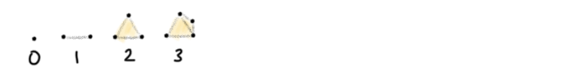
The definition of a simplex is: “a k-simplex is a k-dimensional polytope which is the convex hull of its k + 1 vertices” - Wikipedia. If that is intimidating, it just means that given k independent points, each point/vertex shares an edge with all other verticies. Then create faces, which will be of dimension k-1. Here is a picture of a 0,1,2,3 simplex.
Simplicial Complex
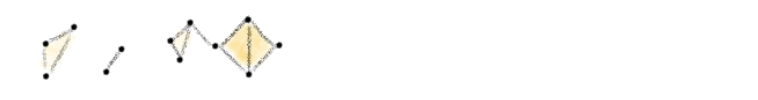
The definition of a simplicial complex is: a set of simplices, K, such that all faces are in the set K, and if there is a non empty intersection between two simplicies from K, it must be a face which is in K - Wikipedia. The first part of the definition is the more defining aspect, the second part ensures you don’t have any weird “interactions” between simplicies (the only “interaction” they can have is sharing a face). As usual, I drew an example of a simplicial complex for you to have a mental representation.
Čech complex
The Čech complex takes in sets, and produces a simplicial complex based on the intersection between sets. It does this by assigning every set a vertex (0 simplex). If n sets have a non-empty intersection, then connect the n 0-simplicies to produce a n-1simplex.
Utilizing the Čech complex
If we have an open cover of a set S we have open sets such that their union contains S. We conflate open covers and Čech complexs and produce a simplicial complex that resembles the original S. For example, imagine S is the letter ‘J’. I have drawn two covers and their corresponding Čech complex. Hopefully you can tell which one is a better representation (it’s the one on the right).
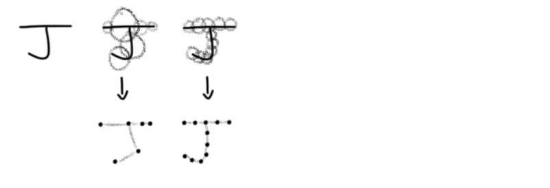
It appears that having uniform sets covering S produces a better representation of S. We will discuss more about this soon.
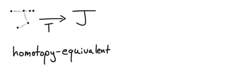
Nerve Theorem
Nerve Theorem formally describes the aforementioned idea. In simple terms, if our covering of S is good, we can get a simplicial complex that is homotopy-equivalent to S. That should be pretty intuitive, other than the homotopy-equivalent, which means by “bending, shrinking and expanding” you can go from S to the simplicial complex and vice versa - Wikipedia.
The Core of UMAP
Local Metrics
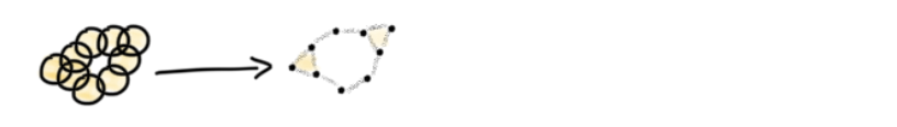
Before I mentioned that having uniform points makes it easier to produce a good simplicial complex. However, real world data is not uniform. UMAP solves this problem by utilizing ideas from Riemannian manifolds. Riemann manifolds can be squished, stretched, and contorted in varying places from a perspective outside of the manifold. For example in some part of a manifold M in 2D say it is locally defined such that moving 1 unit north locally will actually take you 2 units from a global perspective, and in another part moving 1 unit north could take you to .5 units north east globally, it all depends on how the manifold is locally defined. Similarly, a local metric is how distance is defined. To have a visual, look at two possible covers for the topological space.
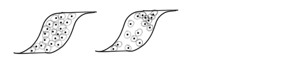
As with the ‘J’ example the on left is clearly better. But imagine we only have the data from the left. How UMAP creates a local metric based on the nearest neighbors for each point. Just by observing the nearest neighbors in the image below we can get an idea on how to define the local metric such that a constant radius from every point will produce a good cover.
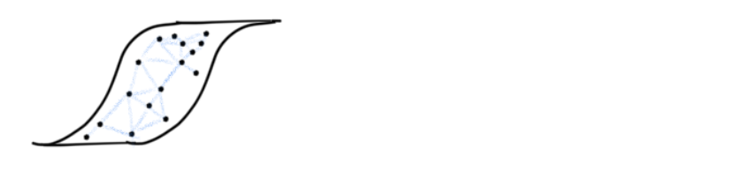
We utilize the nearest neighbors and construct a graph. Furthermore, the authors view edge weights as probabilities. Below are the equations needed to define the local metrics and consequently the edge weights. Note that the edges are directed (from xi to xj).
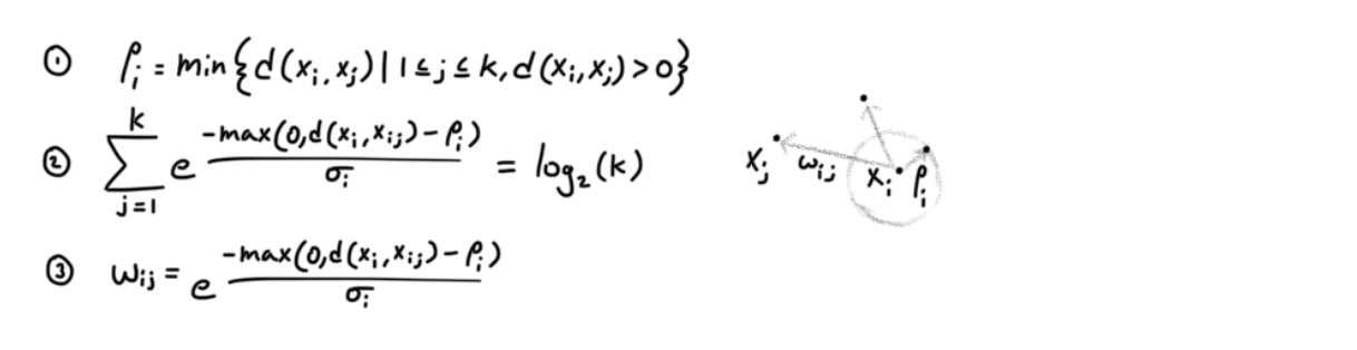
pi is the distance to the closest point and σi is a normalizing factor. Hopefully through these equations you can see how based on the neighboring distances, we define a local metric and discretely shrink/expand space, and the same region can shirnk/expand in multiple ways if it is part of multiple local metrics. The local metric is defined by pi, and σi.
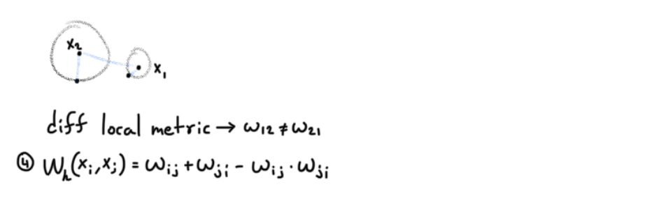
Local Metric Incompatibility
While we can define wij, it doesn’t mean that wij = wji. This is because we didn’t define how to transition between two local metrics. Therefore, based on A’s local metric, the distance from A to B will be different from the distance from B to A using B’s local metric. Because the directed edge weights can be viewed as probabilities, the authors combine wij and wji by the following formulas. In short they take the union of wij and wji.
Graph Embedding
Our final problem is embedding this graph into a low dimensional space such that as much of the topology is preserved. To measure how much of the structure is captured the authors utilize cross entropy as a loss function to measure the distance between both the high dimensional and low dimensional graph.
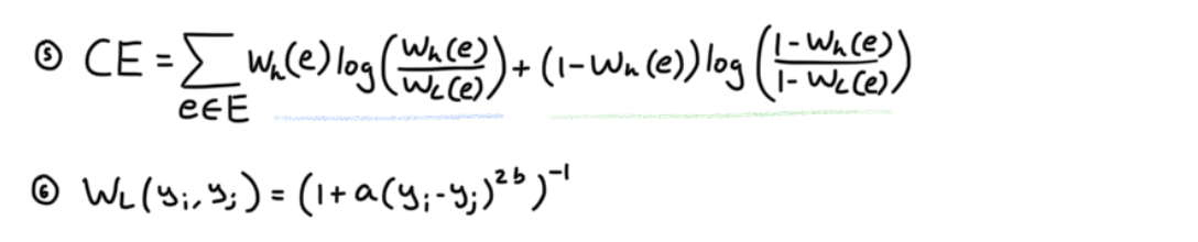
WL is a distance metric which I will explain shortly. The authors say that cross entropy loss acts like a force directed graph layout algorithm, where pushing and pulling different points via their edges will manipulate the low dimensional graph into one that preserves as much of the topological structure of the high dimensional graph. To see why this works, I illustrated the following example.
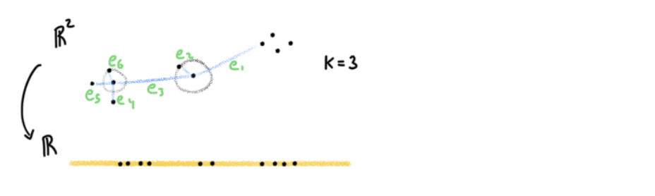
I didn’t draw all the edges for simplicity. Nevertheless, if you can see why e6’s vertices will be closer than e3’s, then you can apply the same logic to all points. e6 will be greater than e3 due to how edge weights are defined (equation 4). Therefore, looking at the blue section, we know that will be weighted more than the blue section’s
. Going to geen’s log, it will be minimized when WL(e6) is as large as possible, and by equation 6, that occurs when the euclidean distance is small. Therefore this is the attractive force. For points with high weights in the high dimensional graph like e6, this attractive force is stronger than the repulsive force due to Wh(e) > (1-Wh(e)). The repulsive force is defined by
. So to summarize, higher weighted edges have a stronger attractive force, and lower edge weights edges have a stronger repulsive force. By gradient descent we can find the right lower dimensional graph that optimizes for this pulling and pushing act.
Why a Simple K Nearest Neighbor Graph isn’t Used
It is the curse of dimensionality that makes the k nearest neighbor distances in high dimensions very similar. The following image shows how as you increase the dimensions, the distance distribution’s mean increases and its variance decreases.
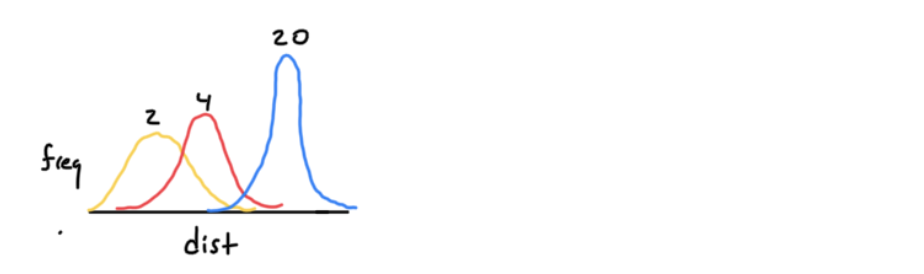
There is math to show that the UMAP process stretches the distribution out, which is very useful.
References
https://arxiv.org/pdf/1802.03426.pdf
https://www.youtube.com/watch?v=nq6iPZVUxZU&t=0s
https://umap-learn.readthedocs.io/en/latest/how_umap_works.html
https://www.youtube.com/watch?v=VPq4Ktf2zJ4
https://www.cs.cornell.edu/courses/cs4780/2018fa/lectures/lecturenote02_kNN.html