Policy Gradients

I previously explained QLearning. While it is a key concept with more powerful extensions such as Deep-Q Learning, policy gradients are a different approach that has its benefits. In general, they can generalize better in more complex domains, and this thread contains a good overview of more comparison. In this article, I will first start with vanilla policy gradients, since that lays down the foundations, and then show a variant of it that is more efficient, and finally show an implementation (it didn’t perform that well, but it still learned basic skills).

The Fundamentals

Imagine you have a model that gives you a probability distribution of actions for a given state. How do you compute how good this model is? Let’s look at the following visual.
drawing
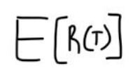
In our finite set of paths, some produce more reward than others which is shown by the shade of green. Therefore, we can evaluate how good our policy is via the following expectation.
drawing
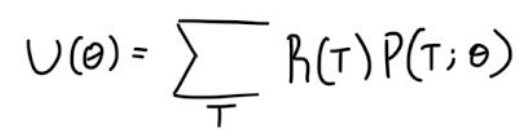
We can rewrite this expectation as
drawing
What we want to do is maximize that expectation, because that would mean our model has found the optimum distribution for each action for a given state, and consequently, the actions that lead to better rewards would have higher probabilities. So one way we can maximize that expression is via gradient descent. Thus, we need to calculate the gradient.
drawing
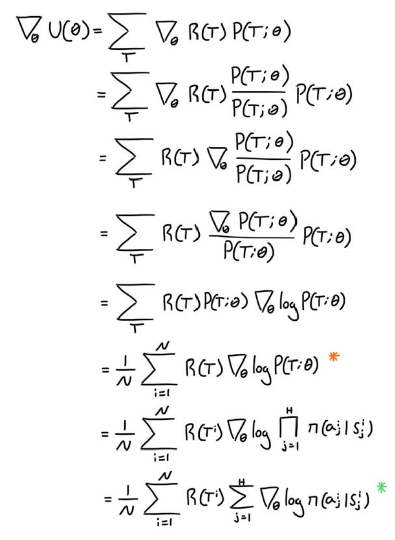
The orange * is the log derivative rule. Therefore we can write the process of applying gradient descent as:
drawing
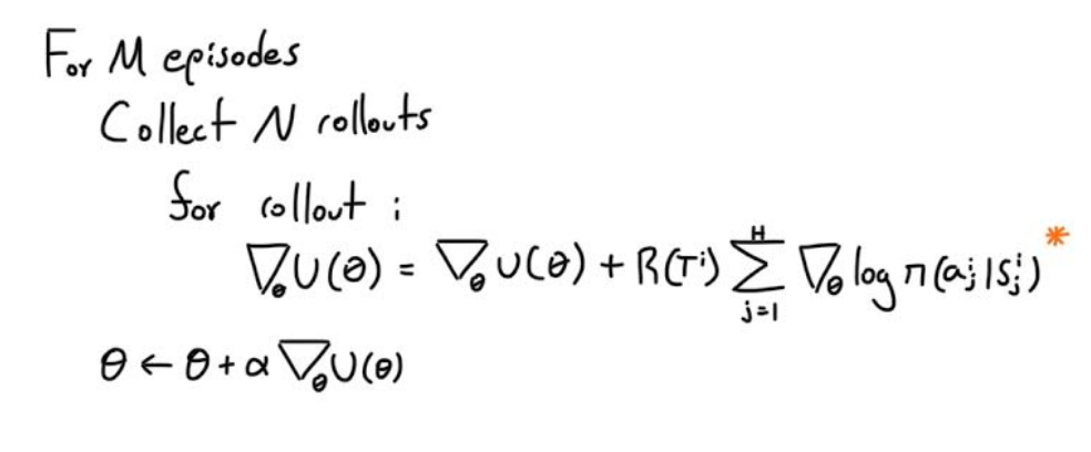
The green star the second orange *, represents one way of treating the reward function, but it’s better to discount our reward at each time step, rather than just summing all of them. So our gradient accumulation would look like the following.
drawing
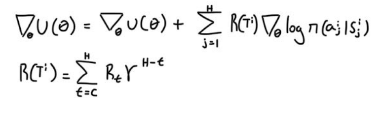
And that’s vanilla policy gradient, this model is called REINFORCE, it lays down the fundamentals which are then optimized via more sophisticated models.

Baseline And How It’s Unbiased

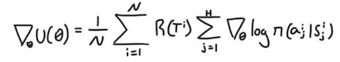
So what if I posit the following equation for the gradient. Where instead of our original equation we now have the following.
drawing
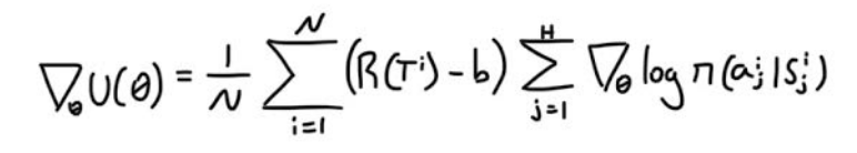
Well, how can I justify editing the reward? We need to show that our new equation for $\nabla U(\theta)$ is equal to our original one. Thus observe the following proof which a modified version of Sergey Levine’s awesome set of slides drawing
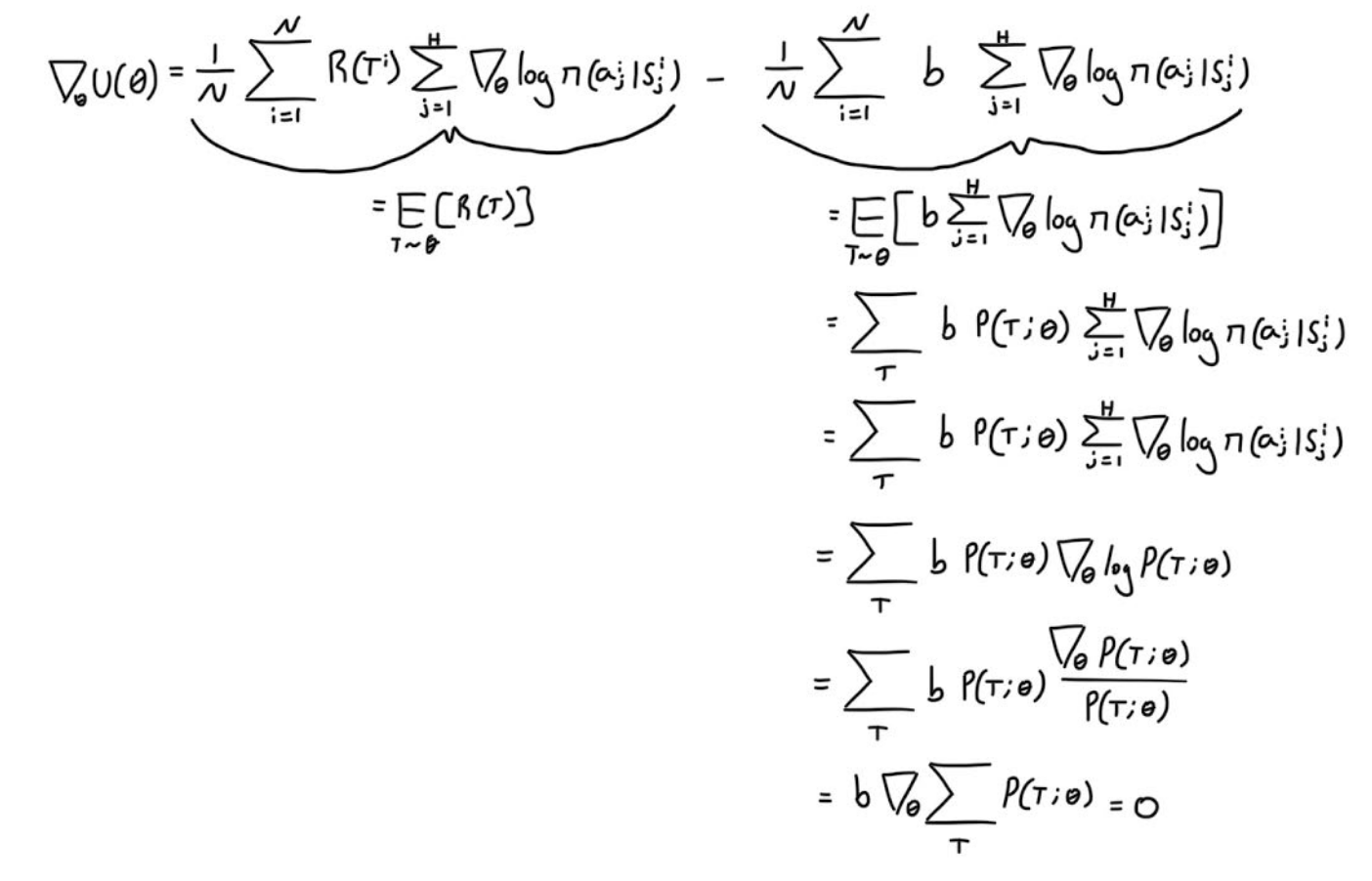
Here we show that our updated equation/estimator for the gradient is the same as our original one, which means that it’s unbiased. So why did I go through this trouble to obtain the same value? Well there is an issue with our original equation for the gradient:
drawing
The issue is its variance. It has a rather high variance, thus we need even more samples to obtain more accurate estimates of our gradient. Thus finding an estimator that is unbiased and has a lower variance would be more efficient. This article is great for explaining why the variance is reduced. Common values for b are E(R(t)) or V(s).

Implementation

I implemented REINFORCE with baseline, for CartPole-v1. While Q-Learning is the go-to for this environment, I thought it would be fun to give policy gradients a try. I made my network output μ and σ for the action. Since CartPole-v1 only takes 0 or 1 as an action, if the sampled value from the network’s distribution was less than .5 then it was considered as 0 and vice versa for 1. I will post the code below. Here is a video of how the model did at episode 10. drawing
The average number of iterations the pole could be balanced was 14.13. After 2180 episodes, the network hit its peak, which is shown by the following video.
drawing
Its average time balanced was 34.41. Therefore there is a clear improvement, however, an actual good score should be around 100+. But we do see the policy pick up some back and forth skills. I should have made my reward discounted, and maybe played around with some hyperparameters, maybe you could modify the code and send me the results :)

Code

Policy Training

import numpy as np
import gym
import torch
import torch.nn as nn
import torch.nn.functional as F
import torch.optim as optim
from time import sleep
from torch.distributions import MultivariateNormal

class Policy(nn.Module):
	def __init__(self,stateSize):
		super(Policy, self).__init__()
		self.f1 = nn.Linear(stateSize,8)
		self.f2 = nn.Linear(8,4)
		self.f3 = nn.Linear(4,2)
		self.mu = nn.Linear(2,1)
		self.std = nn.Linear(2,1)

	def genParameters(self,s):
		x = torch.tanh(self.f1(s))
		x = torch.tanh(self.f2(x))
		x = torch.tanh(self.f3(x))
		mu = torch.tanh(self.mu(x))
		std = torch.sigmoid(self.std(x)).view(1,-1)
		return(mu,std)

	def logPrb(self,a,mu,std):
		dist = MultivariateNormal(mu,std)
		return(dist.log_prob(a))

	def sampleAction(self,s):
		mu,std = self.genParameters(s)
		dist = MultivariateNormal(mu,std)
		return(dist.sample())

	def forward(self,a,s):
		mu,std = self.genParameters(s)
		return(self.logPrb(a,mu,std))

def rollouts(n):
	rewards = []
	baseline = 0
	stateActionPairs = []
	for itter in range(n):
		obs = env.reset()
		currPair = []
		currReward = 0
		done = False
		while not done:
		
			action = policy.sampleAction((torch.from_numpy(obs).float().to(device))).item()
			if(action >.5):
				action = 1
			else:
				action = 0
			obs, reward, done, info = env.step(action) 
			currReward += reward
			currPair.append((obs,action))
		rewards.append(currReward)
		baseline += currReward
		stateActionPairs.append(currPair)
		done = False
	return(stateActionPairs, rewards, baseline/float(n))

device = torch.device("cuda:0" if torch.cuda.is_available() else "cpu")
policy = Policy(4)
policy.to(device)
env = gym.make("CartPole-v1")

n = 200
numEpisodes = 3000
PATH = 'cartPole_checkpoints/'
optimizer = optim.Adam(policy.parameters(), lr=1e-3)

for episode in range(numEpisodes):
	stateActionPairs,rewards,baseline = rollouts(n)
	optimizer.zero_grad()
	loss = 0
	for i in range(n):
		reward = rewards[i]
		for j in range(len(stateActionPairs[i])):
			action = torch.tensor(([stateActionPairs[i][j][1]])).float().to(device)
			state = torch.from_numpy(stateActionPairs[i][j][0]).float().to(device)
			loss += -1*(reward-baseline)*policy(action,state)
	loss = loss/float(n)
	loss.backward()
	optimizer.step()

	print(episode,baseline)

	if(episode%10 == 0):
		torch.save(policy.state_dict(), PATH+str(episode)+".pt")


print('Finished Training')

Running the policy

import numpy as np
import gym
import torch
import torch.nn as nn
import torch.nn.functional as F
import torch.optim as optim
from time import sleep
from torch.distributions import MultivariateNormal

class Policy(nn.Module):
	def __init__(self,stateSize):
		super(Policy, self).__init__()
		self.f1 = nn.Linear(stateSize,8)
		self.f2 = nn.Linear(8,4)
		self.f3 = nn.Linear(4,2)
		self.mu = nn.Linear(2,1)
		self.std = nn.Linear(2,1)

	def genParameters(self,s):
		x = torch.tanh(self.f1(s))
		x = torch.tanh(self.f2(x))
		x = torch.tanh(self.f3(x))
		mu = torch.tanh(self.mu(x))
		std = torch.sigmoid(self.std(x)).view(1,-1)
		return(mu,std)

	def logPrb(self,a,mu,std):
		dist = MultivariateNormal(mu,std)
		return(dist.log_prob(a))

	def sampleAction(self,s):
		mu,std = self.genParameters(s)
		dist = MultivariateNormal(mu,std)
		return(dist.sample())

	def forward(self,a,s):
		mu,std = self.genParameters(s)
		return(self.logPrb(a,mu,std))

policy = Policy(4)
policy.load_state_dict(torch.load("cartPole_checkpoints/2180.pt"))
#policy.load_state_dict(torch.load("cartPole_checkpoints/10.pt"))
policy.eval()

env = gym.make("CartPole-v1")
obs = env.reset()
done = False
average = 0
n = 100
for i in range(n):
	rewards = 0
	done = False
	while not done:
		action = policy.sampleAction((torch.from_numpy(obs).float())).item()
		if(action >.5):
			action = 1
		else:
			action = 0
		obs, reward, done, info = env.step(action)
		rewards += reward
		env.render()
		sleep(.03)
	print(rewards)
	average += rewards
	done = False
	obs = env.reset()

print("average:",average/n)

References

Deep RL Bootcamp Lecture 4A: Policy Gradients
http://rail.eecs.berkeley.edu/deeprlcourse-fa17/f17docs/lecture_4_policy_gradient.pdf
https://danieltakeshi.github.io/2017/03/28/going-deeper-into-reinforcement-learning-fundamentals-of-policy-gradients/